Nyquist Plot (Polar Locus)

Abstract

We know that for an open loop system we can define it as : $GH$ and the values that cause GH to go to infinity are poles. We also know that if there are any poles in the Right Hand Plane that the system is unstable

We also know that we can define our closed loop as:

$$\frac{1}{1+GH}$$

And that the zeros of $1+GH$ cause the overall Closed Loop TF to go to infinity. Therefore if there is a zero in $1+GH$ residing in the RHP, the CL TF is unstable.

The problem is, adding $1$ to $GH$ changes the root locus significantly:

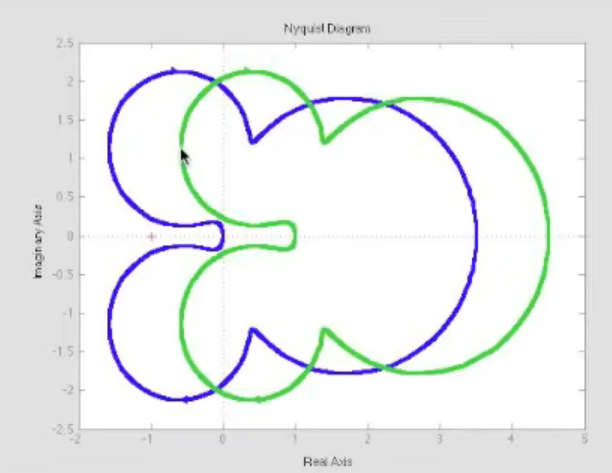
Adding 1 to a Nyquist Plot however simply shifts it:

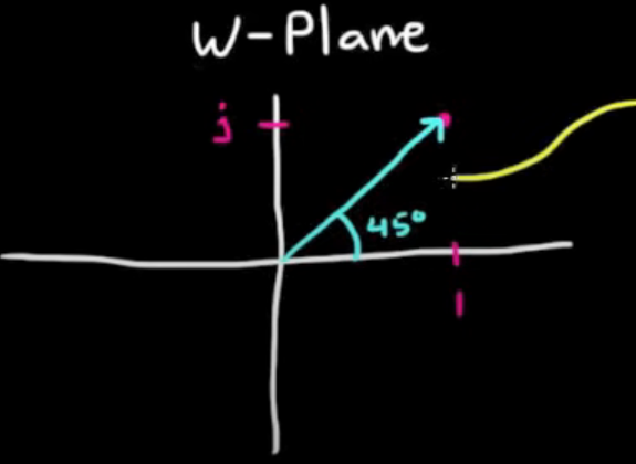
So the general idea is, that we can take any point, and map it against our transfer function: i.e $-1+j$ mapped against $\frac{s+2}{s+1}=1-j$ . This is no longer in our $s$ plane but rather a new $w$ plane.

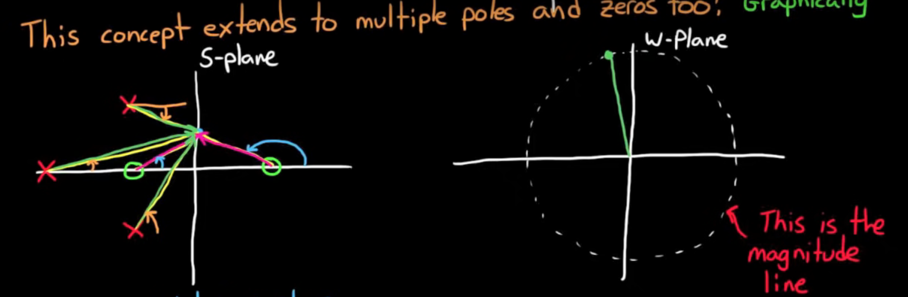
A quick math aside: The phasor between the point selected and the zero in the $s$ plane is the same as the phasor from the origin to the point in the $w$ plane:

					![[Pasted image 20240422143120.png|200]]

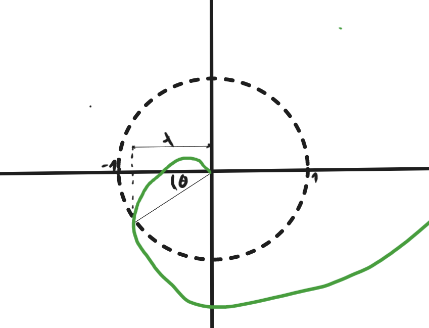
This concept even extends to multiple zeros. Now the interesting thing with this is that we will not make a full circle unless our point selected goes around (encircles) a root or zero. The circles in the W plane will encircle the $-1$ point (remember $1+GH$):

• Counterclockwise for each pole
• Clockwise for each zero

The point rises then, that if we have an equal amount of zeros and poles in the RHP, how do we know stability? This is easily done by checking the stability of the OL TF ($GH$), which if it is stable, and there is no encirclements of the $-1$ point of the $w$ plane, we know for a fact our CL is stable. This is called the Nyquist Stability Theorem

That is, this applies for a special type of s plane region, called the Nyquist Contour, which encircles the entire RHP, meaning that we can derive the w plane for the stability of the system.

Deriving Gain and Phase Margins

Phase Margin: $-180+\theta$ Gain Margin: $\frac{1}{\lambda }$

TL;DR

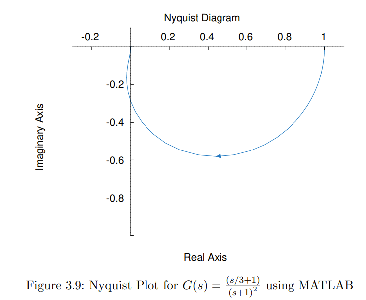
The polar locus is a graph showing how the phase and magnitude of the frequency response varies with frequency, $\omega$.

Extra

Basic Steps:

1. Determine the behavior of the magnitude and phase as $\omega \to 0$:
   1. If the transfer function has no integrators (i.e. no poles in the origin), then the phase is 0 and the magnitude can be calculated by setting $\omega =0$.
   2. If the transfer function has $N$ pure integrators (i.e. $N$ poles in the origin), then the magnitude at $\omega =0$ is $\infty$, while the phase is $-90^o\ast N$).
2. Determine the behaviour of the magnitude and phase as $\omega \to \infty$. The phase is determined by the relative order of the system 3 . For all real systems the number of poles is larger than the number of zeros, so the relative order $(n-m)>0$). This means that, as $\omega \to \infty$,
   1. the phase is $\arg G(j\omega )=-90^o\ast (n-m)$
   2. the magnitude is $|G(j\omega )|=0$

Examples

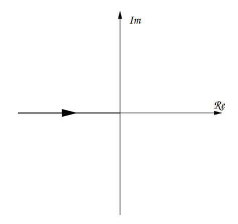
Simple Integrator

The simple integrator is defined as: $G(s)=\frac{1}{s}$

This results in the frequency response form of: $G(j\omega )=\frac{1}{j\omega }$

Which can be seen to have a constant phase of $-90^o$ and a magnitude of: $|G(j\omega )|=\frac{1}{\omega }$

The corresponding plot would be:

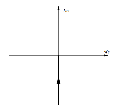
Double Integrator

The simple integrator is defined as: $G(s)=\frac{1}{s^2}$

This results in the frequency response form of: $G(j\omega )=\frac{1}{(j\omega {)}^2}$

Which can be seen to have a constant phase of $-180^o$ and a magnitude of: $|G(j\omega )|=\frac{1}{(\omega {)}^2}$

The corresponding plot would be:

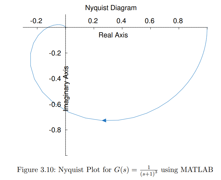
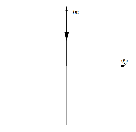
Triple Integrator

The simple integrator is defined as: $G(s)=\frac{1}{s^3}$

This results in the frequency response form of: $G(j\omega )=\frac{1}{(j\omega {)}^3}$

Which can be seen to have a constant phase of $-270^o$ and a magnitude of: $|G(j\omega )|=\frac{1}{(\omega {)}^3}$

The corresponding plot would be:

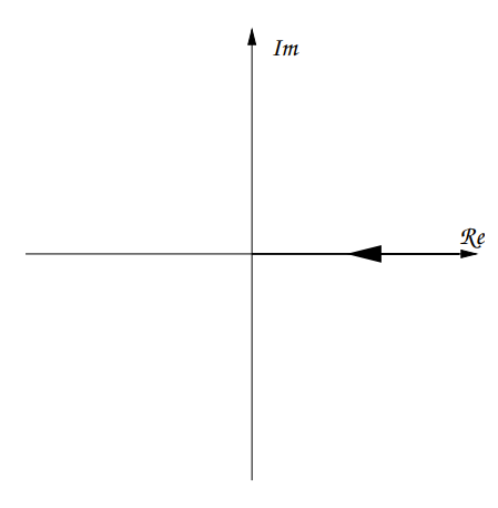
Quadruple Integrator

The simple integrator is defined as: $G(s)=\frac{1}{s^4}$

This results in the frequency response form of: $G(j\omega )=\frac{1}{(j\omega {)}^4}$

Which can be seen to have a constant phase of $-360^o=0^o$ and a magnitude of: $|G(j\omega )|=\frac{1}{(\omega {)}^4}$

The corresponding plot would be:

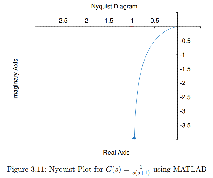
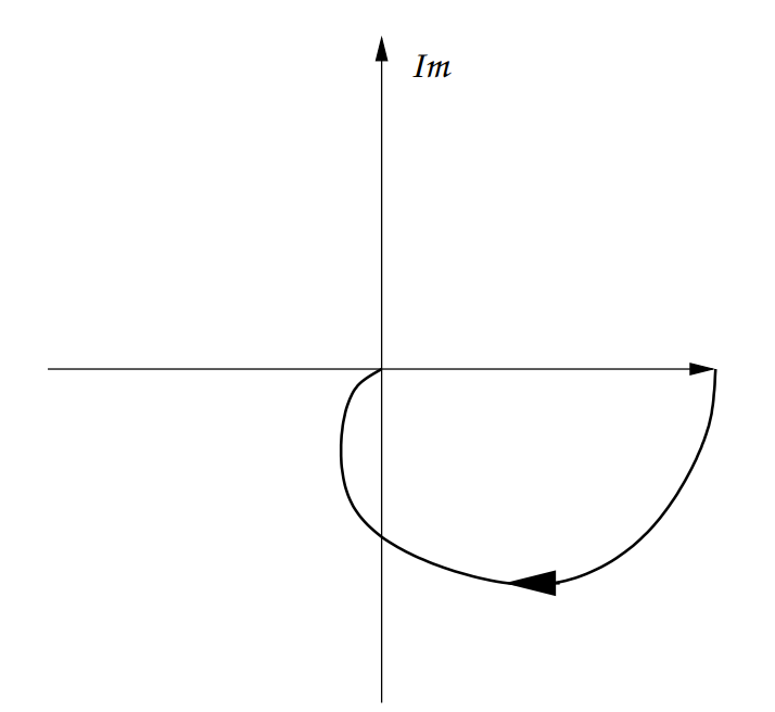
Simple Lag

The simple integrator is defined as: $G(s)=\frac{1}{s/{\omega }_c+1}$

This results in the frequency response form of: $G(j\omega )=\frac{1}{1+(j\omega )/{\omega }_c}$

Which can be seen to have

• a phase of $-{\tan }^{-1}(\omega /{\omega }_c)$, This varies between ($0$ when $\omega =0$) and ($-90^o$ as $\omega \to \infty$)
• and a magnitude of: $|G(j\omega )|=\frac{1}{\sqrt{1+{\omega }^2/{\omega }_c^2}}$, This varies between ($1$ when $\omega =0$) and ($0$ as $\omega \to \infty$)

The corresponding plot would be:

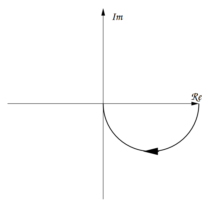
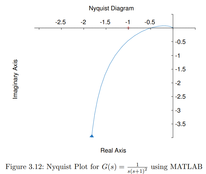
Double Lag

The simple integrator is defined as: $G(s)=\frac{1}{(s/{\omega }_c+1{)}^2}$

This results in the frequency response form of: $G(j\omega )=\frac{1}{(1+(j\omega )/{\omega }_c{)}^2}$

Which can be seen to have

• a phase of $-2{\tan }^{-1}(\omega /{\omega }_c)$, This varies between ($0$ when $\omega =0$) and ($-180^o$ as $\omega \to \infty$)
• and a magnitude of: $|G(j\omega )|=\frac{1}{1+{\omega }^2/{\omega }_c^2}$, This varies between ($1$ when $\omega =0$) and ($0$ as $\omega \to \infty$)

The corresponding plot would be:

Other Specific Plots:

$G(s)=\frac{1}{(s+1{)}^2}$ / Double Lag

$G(s)=\frac{(s/3+1)}{(s+1{)}^2}$

$G(s)=\frac{1}{(s+1{)}^3}$ / Triple Lag

$G(s)=\frac{1}{s(s+1)}$

$G(s)=\frac{1}{s(s+1{)}^2}$