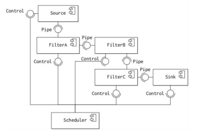
The pipe and filter architectural pattern addresses these design problems by leveraging the homogeneous format of the data being processed. The diagram illustrates the basic form of the pattern.
- Each transformation that must be applied to the data is implemented as a single component called a filter. Each filter provides and implements the same interface, sometimes called the pipe. The filters are then wired into a single sequential assembly called the pipeline, with each successive component obtaining data from a component on the left and passing output to the component on the right.
- Two special components bound the pipeline. A data source component provides input on the right and requires the pipe interface. Similarly, a data sink component provides the pipe interface on the right to accept the system’s output on the right.
- Finally, a Scheduler component is responsible for deciding which of the other components should execute at anyone time. The Scheduler’s job is to manage load between the other components so that no one component causes a bottleneck in the pipeline. The Scheduler controls each component via the Control interface.
- The pattern satisfies the design problems described above because:
- Processor time is allocated to the different filters based on load. This ensures an even flow of data through the pipeline.
- All of the filters provide and require exactly one pipe interface, so can be re-ordered and composed as necessary.
Variants to the basic pipe and filter model
- Push or Pull Data Flow
- Sequential or concurrent data processing
- Re-orderable vs. Inter-changeable filters
- Branching Filters
Push or Pull Data Flow
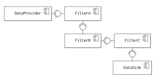
The push or pull driven data flows reflect two different controlling processes for moving data to the pipeline, as illustrated in Figure the diagram.
In the push model, data is driven into the system by an active DataProvider, which submits the data to FilterA for processing. The DataProvider will continue to supply data to the filter, until the Filter is blocked by a full buffer. FilterA will process the data and then pass the results on to FilterB. This process continues until the data is written out to a passive DataSink by the last filter.
The pull model is the reverse of this situation. The DataRequester actively polls the last filter, FilterC for data. FilterC polls FilterB in turn and the process continues until the last filter polls the DataSource for data to process. The results are then passed back along the request pipeline. The choice of which data model to employ depends on the system for which the application is to be used:
- A push data model is appropriate when the data to be processed is being continually generated in an unpredictable or continual way by the Provider. This means that the data is fed into the pipeline as and when it becomes available. Multi-media format conversion of an entire media file, or of a continual live stream is a good example of this situation.
- A pull data model is more appropriate when data needs to be processed as a result of some external event in the data Requester. The Requester only initiates the pipeline when it needs the data to be processed. Execution of a scientific experiment that integrates a large collection of diverse data sets is a good example of this situation.
Sequential or concurrent data processing
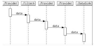
The data can also be processed in different ways within each individual filter. The diagram illustrates the two variants using a push-style pipeline, as described above.
In a sequential pipeline, all the data submitted to the pipeline is processed by each filter in turn, before the data is passed on to the next filter. This means that processing is serialised: the total time taken to process

In a concurrent pipeline, small amounts of data (often called chunks for text, or blocks for raw bytes) are fed into the pipeline as soon as they become available. This means that the data sink receives the first blocks of data as soon as they are processed by the last filter.
At first glance, it might seem that the concurrent model is always better, since it means that data begins arriving at the data sink earlier and if the system is distributed on a number of processing nodes the overall computation should end more quickly. This may be important for certain applications that require a constant stream of data to be written to the data sink (live video streaming for example).
However, there are many applications where it is better to process larger blocks of data in one go. Compression algorithms, for example, generally achieve a greater compression ratio (the size relationship between the raw and uncompressed data) if they are executed on larger blocks of data.
Informally, this is because the probability of redundancy (repeated data) increases as the size of the data block increases.*
In practice, this means that there is a trade-off between speed of execution and performance, made in terms of the size of data block operated on in the pipeline.
Re-orderable vs. Inter-changeable filters
Another decision to made when designing a pipeline architecture or framework is the extent of flexibility that will be permitted to a pipeline constructor. Two possible variants are re-orderable or interchangeable filters.
- The most flexible option is to allow the filters to be re-ordered as desired by the software architect. To enable this arrangement, every single filter must provide and require the same interface.
- This flexibility means that the overall processing pipeline can be optimised by re-ordering processing activity.
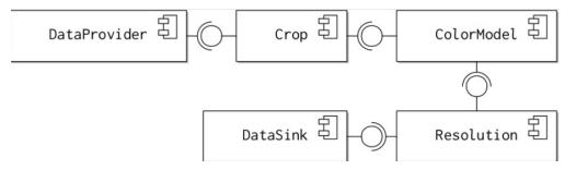
For example, in a video processing application it is quicker to crop each video frame and then convert them to grey scale, as shown in the diagram. If the reverse configuration is employed, computation time is wasted converting regions of each frame to grey scale that will be removed anyway
A more restrictive option is to fix the ordering of filters and only permit the inter-change of filter implementations. In this case, each filter can provide and require different interfaces. Any filter can be replaced by another filter implementation that provides and requires the same interfaces. However, the heterogeneous nature of the filter interfaces means that they cannot generally be re-ordered.
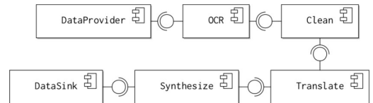
Consider, for example: An application for converting a scanned image of a page of book into audible speech in another language, as shown in the diagram.
The filters of the system might be:
- optical character recognition;
- spell check;
- grammar check;
- text translation;
- speech synthesizer.
These components cannot be re-ordered and each filter requires a different form of input data. However, the implementation of each component can be swapped as required.
Again, it is possible to compromise between these two architectures, so that some parts of the pipeline can be re-ordered, while others require set sequences of filter types.
Branching Filters
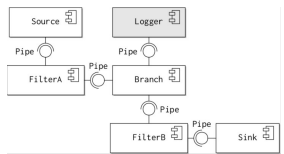
A final variant is to allow the use of branching filters in the pipeline, as shown in the diagram. A branching filter can do one of two things with incoming data:
- Replicate the data stream to the out-going filters;
- Filter each data item into one of the out-going branches.
Branches can be useful in pipelines for several reasons:
- Performing ancillary functions on exact copies of data, e.g. logging intermediate versions of a data set during a computation for debugging, verification or auditing purposes. This means that these functions do not have to be built into the filters themselves.
- Applying two different transformations to the same incoming data source simultaneously. A video stream might need to be encoded for high and low quality distribution, for example.
- Separating data items into different categories for alternative processing. A data stream might contain words in two different languages that need to be separated and processed differently, for example