Interrupt Questions
Entering an Interrupt:
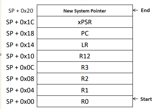
- Update your Stack:
- Load xPSR, PC, LR, R12, R3, R2, R1, R0 to the stack (You’re expected to know these values)
- Update your stack pointer by SUBTRACTING 8 registers x 4 bits = 32 bits (0x20)
- Identify your Exception from your Exception Vector Table:
- For the general form: IRQn. The exception number is 16+n, and the offset is 0x40+4n
- Update your PC:
- Set PC to the value of your exception (you’re usually given a table w/ exception no.)
- Update your LR:
- Here’s a flowchart:
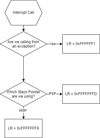
- Here’s a flowchart:
- Update your xPSR:
- Add your Exception Number in hex to your current xPSR
- Change the Mode to Handler:
Sample Question (Tutorial 2 2023)
Abstract
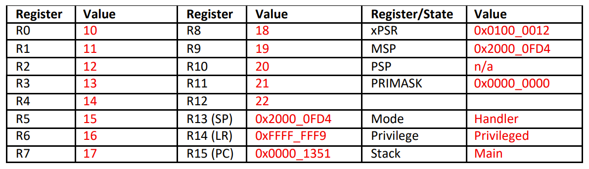
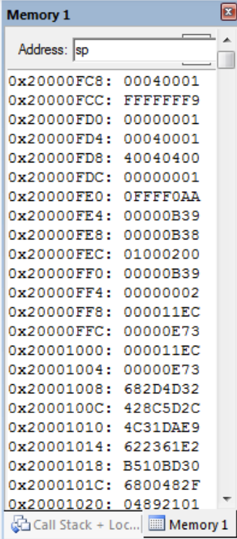
Fill in the following table to show the contents of memory and registers after the CPU responds to an IRQ2 exception request, but before it executes any code in the interrupt.
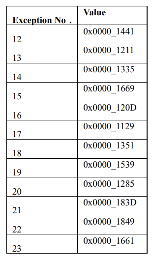
You are also provided with the following table of Exception Values:
Example
- We load xPSR, PC, LR, R12, R3, R2, R1, R0 onto the stack, and then we update our SP:
- SP = 0x2000_0FF4 - 0x20 = 0x2000_0FD4
- (We also need to update MSP to the same value)
- We identify our exception:
- IRQ2 exception means Exception No 16+2 = No 18.
- We update our PC:
- From the table we can see No 18 corresponds to 0x0000_1351
- PC = 0x0000_1351
- We update our LR:
- We are calling this operation from the main thread, and we are using the MSP
- LR = 0xFFFF_FFF9
- We update our xPSR:
- xPSR = 0x1000_0000 + 0x12 (18 in hex) = 0x1000_0012
- We update our mode to handler :
Exiting an Interrupt:
Typically a question on this topic will add an extra POP command to take into consideration.
Given a POP{R1-R3,LR} command, you will have to show that the stack will pop:
The first 4 items on the stack,
- R1
- R2
- R3
- LR Before proceeding to:
- R0
- R1
- R2
- R3
- R12
- LR
- PC - (Return Address)
- xPSR
You will then identify how many items have been popped from the stack:
In this case the standard 8 + 4 defined in pop. And then ADD 12 items * 4 bits = 48 bits to the SP:
SP = SP + 0x30;
Your “Return Address” will be the PC popped just before the end. Which I have labelled
You may even have to specify the offset of each one as such:
Sample Question (Tutorial 2 2023)
Abstract
What is the return address will an exception handler return to, given the following register and memory contents? Assume the instruction for exiting the exception handler is POP {R4,PC}.
Example
Therefore our Return Address is 0x0000_0B38, Stored at the address 0x2000_0FE8
General Interrupt Questions:
Percentage of time spent in Interrupt:
Minimum Main Loop Update Rate:
Assembly
Instructions:
Abstract:
Instructions are in the form:
COMMAND Destination Register, Parameter 1, Parameter 2
Where there might not be a second parameter
Or the form:
COMMAND Register, [Stack Pointer, #offset]
Where the offset is taken from the initial stack pointer from the start of the function as this doesn’t dynamically change mid function
Or finally:
COMMAND Register, |Lx.xx|
Where |Lx.xx| points to a value in a literal pool (just a place in memory full of preset values basically)
Common Instructions:
Instructions involving Registers
MOV:
For the context of this course:
MOV R1,R2 “moves” the value of R2 into R1
Essentially R1 := R2
MOVS:
For the context of this course:
MOVS R2,#0xf moves a static/arbritary size value into a register
Essentially R2 := 0xf
Arithmetic Instructions:
Instructions like ADD, SUB, MULS are all relatively simple and self explanatory commands in the form of:
COMMAND Destination Register, Parameter 1, Parameter 2
MVNS:
MVNS R1,R0 moves the two’s complement (the negative representation) of a register into another
Essentially R1 = -R0
Instructions involving the Stack & Registers
STR:
This command of the form:
STR Register,[sp,#offset]
Is used to store the value of the selected register on the stack at a certain offset. it DOES NOT alter the value of SP
LDR:
This command of the form:
LDR Register,[sp,#offset]
Is used to load the value of the stack (at a certain offset from the SP) into a register. it DOES NOT alter the value of SP
PUSH:
This command takes the form:
PUSH {RegisterX-RegisterY}
OR
PUSH {RegisterX,RegisterY}
Or a combination of the two.
The command will push the value(s) specified onto the stack, typically in the order specified (i.e left to right) and it will also UPDATE THE STACK POINTER accordingly
POP:
This command takes the form:
POP {RegisterX-RegisterY}
OR
POP {RegisterX,RegisterY}
Or a combination of the two.
The command will pop the value(s) specified off the stack, typically in the order specified (i.e left to right) and it will also UPDATE THE STACK POINTER accordingly
For this command, you dont need to specifically think about the relevance of the values being popped, just the order of the items.
You will notice often that you will get values such as PC, LR, R12, and R0-3 all popped off the stack before a function return, where you also pop those values off the stack, however these are different values, and popping something like PC before a function return doesn’t change the way you return from the function.
Other Instructions:
Branching
BL (sometimes BL.X):
Branch and Link, as the name implies, is the Instruction that calls a “function”, typically specifying the address of said function, as well as setting the link register to the next instruction after the BL command so that the program can return
Essentially, go to that function and come back when you’re done
BX
This is called at the end of subroutines/functions and tells the function to return to the location specified (Typically the Link Register)
Essentially, go back to the function you were called from
B :
Branch, is essentially: Go to that function and don’t come back
Conditional Branching:
Typically these command come directly after a CMP RegisterX, RegisterY command
BLO:
Go to this function if (Branch Lower)
BLS:
Go to this function if (Branch Lower or Same)
BEQ:
Go to this function if (Branch Equals)
BHS:
Go to this function if (Branch Higher or Same)
BHI:
Go to this function if (Branch Higher)
BNE:
Go to this function if (Branch Not Equal)
Extra on Instructions:
Instructions using memory will sometimes include the letter B after them, specifying that they are only operated on a single byte, this is for efficiency Instructions with an additional H specify half word
Timer/Counter
Abstract
A counter is the fundamental hardware element found inside a timer.
You can alter the range from where a counter resets to 0 using the Reload Register. This can be used for numerous things, such as square waves:
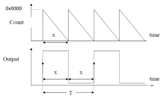 For instance for a Square/PWM signal of period T, you would need to have your counter reload every T/2
So if you know the clock frequency you can calculate how many clock cycles you need for each T/2 and then load this value in hex into your reload register
Example 1:
Abstract
If the max value of a 32-bit down-counter is 0x003A4391 and the bus clock frequency is 10 MHz, How can a pulse-width modulation of 50% Duty Cycle signal with 20 ms period be generated in this system?
Example
As our system runs a 10MHz clock, we can say each counter step takes . So to achieve a PWM signal of period, we can set our reload register to happen every T/2. Which in this case would be / = clock cycles. As we are using a down counter. We can load clock cycles into our reload register. Now to convert to hex: First so the highest power to use is …, = 1 … = 8 = 6 … = A = 0 Therefore we need to load 0x000186A0 into our reload register for a 20mS PWM signal
This example also demonstrates how to convert decimal to hex.
Example 2:
Abstract
If the max value of a 32-bit down-counter is 0x003A4391 and the bus clock frequency is 10 MHz, what is the interrupt period?
Example
| 0 | 0 | 3 | A | 4 | 3 | 9 | 1 |
| Therefore our counter can handle cycles. | |||||||
| Assuming each count happens once per clock cycle: | |||||||
| The interrupt period is |
Endians
Little Endian
This means the “Little End” of the data (i.e. LSB) is stored in the first 8 bits The timer/counter is typically an N-bit up-counter but may sometimes be a down-counter.
Big Endian
This means the “Big End” of the data (i.e MSB) is stored in the last 8 bits
Example:
Abstract
Illustrate how 0x7E5CA4D1 are saved in the memory in both Little and Large Endian formats
Example
Little Endian: Firstly lets split this into bytes 7E - MSB 5C - 2nd Most A4 - 3rd Most D1 - LSB Therefore we can say the data is saved as following in memory 7E = 0111_1110 = MSB 0xFFFF_FFFF 5C = 0101_1100 = 2nd A4 = 1010_0100 = 3rd D1 = 1101_0001 = LSB 0x0000_0000
Big Endian: Firstly lets split this into bytes 7E - LSB 5C - 3rd Most A4 - 2nd Most D1 - MSB Therefore we can say the data is saved as following in memory D1 = 1101_0001 = LSB 0xFFFF_FFFF A4 = 1010_0100 = 3rd 5C = 0101_1100 = 2nd 7E = 0111_1110 = MSB 0x0000_0000
Architecture
Harvard vs Von Neumann
| VON NEUMANN ARCHITECTURE | HARVARD ARCHITECTURE |
|---|---|
| Same physical memory address is used for instructions and data. | Separate physical memory address is used for instructions and data. |
| There is common bus for data and instruction transfer. | Separate buses are used for transferring data and instruction. |
| Two clock cycles are required to execute single instruction. | An instruction is executed in a single cycle. |
| It is cheaper in cost. | It is costly than Von Neumann Architecture. |
| CPU can not access instructions and read/write at the same time. | CPU can access instructions and read/write at the same time. |
| It is used in personal computers and small computers. | It is used in micro controllers and signal processing. |
| (Taken from geeksforgeeks) |
RISC vs CISC
| RISC | CISC |
|---|---|
| Focus on software | Focus on hardware |
| Transistors are used for more registers | Transistors are used for storing complex Instructions |
| Fixed sized instructions | Variable sized instructions |
| Can perform only Register to Register Arithmetic operations | Can perform REG to REG or REG to MEM or MEM to MEM |
| Requires more number of registers | Requires less number of registers |
| Code size is large | Code size is small |
| An instruction executed in a single clock cycle | Instruction takes more than one clock cycle |
| An instruction fit in one word. | Instructions are larger than the size of one word |
| RISC is Reduced Instruction Cycle. | CISC is Complex Instruction Cycle. |
| The number of instructions are less as compared to CISC. | The number of instructions are more as compared to RISC. |
| It consumes the low power. | It consumes more/high power. |
| RISC required more RAM. | CISC required less RAM. |
| (Again abridged from geeksforgeeks) |
Scheduling
Scheduling’s main priority: maximise CPU utilisation, and reduce average waiting times of tasks.
Abstract:
Non-Preemptive.
- In a non-preemptive scheduler, a task will run until completion, and the scheduler is unable to forcibly take away CPU control from the task Pre-Emptive.
- In a preemptive scheduler, a task will typically be ran for a certain period of time before being revoked CPU control by the scheduler, who will reallocate to a different task (this is normally done by time quantums)
Pros of Preemptive:
Preemptive scheduling allows microcontrollers to promptly respond to time-sensitive tasks or interrupts, which is crucial in embedded systems. Time-sharing aspects of preemptive scheduling ensure that lower-priority tasks are not starved of CPU time. In real-time systems, where meeting timing constraints is critical, preemptive scheduling can ensure that high-priority tasks meet their deadlines.
Non-Preemptive Algorithms:
First-Come First-Served (FCFS) :
Algorithm:
- Processes are added to a queue in order of arrival
- Picks the first process in the queue and executes it
- If the process needs more time to complete it is placed at the end of the queue Details:
- Simple to implement
- However, average waiting time can be quite high
Abstract
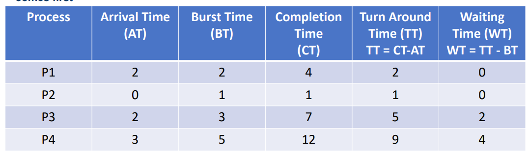
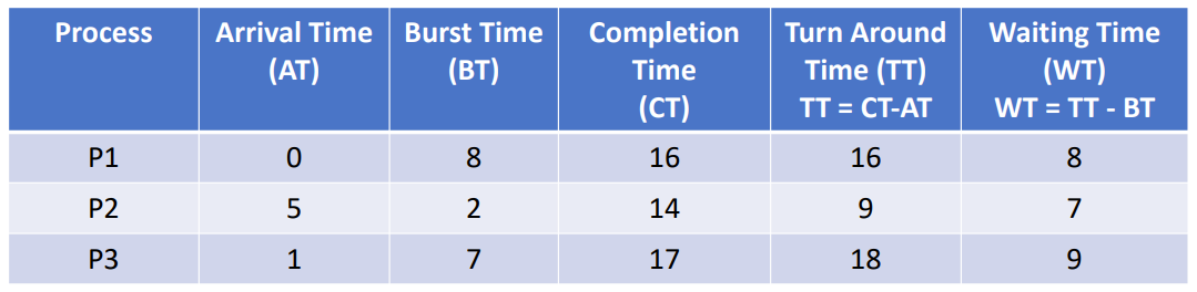
Given the following table:
Calculate the:
- Completion Time
- Turn Around Time
- Waiting Time
Example
First we can work through and create a relative time graph: At:
- t=0 The only ready process is P2, so we run P2 until completion
- t=1 P2 is now finished, but nothing else is ready
- t=2 P1 and P3 have now arrived, P1 will get priority here just by the way we have defined them. P1 runs until completion
- t=4 P1 is now finished, in the mean time P4 has arrived, but P3 takes priority and is run until completion
- t=7 P3 is now finished, we can run P4 until completion
- t=12 P4 is now finished
From this we can extend our table as such:
Shortest Job First (SJF) :
Algorithm:
- Processes are added to a queue, ordered by (next) CPU burst time
- Picks the first process in the queue and executes it
- If multiple processes have the same CPU burst time, use FCFS among them
Details: - Fairly simple to implement
- Provable minimum average waiting time
- Unfortunately Unrealistic
Earliest Due Date (EDD):
Algorithm:
- Processes all arrive at the same time with known deadlines
- Task with the earlier deadline is started. Details:
- Assumes all processes arrive at the same time, can not cope with new processes
Preemptive Algorithms:
Round-Robin (RR):
Algorithm:
- Pre-emptive version of FCFS
- Processes are added to a queue ordered by their time of arrival
- Picks the first process in the queue and executes it for a time interval (quantum)
- If the process needs more time to complete, it is placed at the end of the queue
- If the process ends before the quantum time, move on to next process in queue Details:
- Quite simple to implement
- May also lead to long waiting times
- Performance depends heavily on the length of the time slice
Example
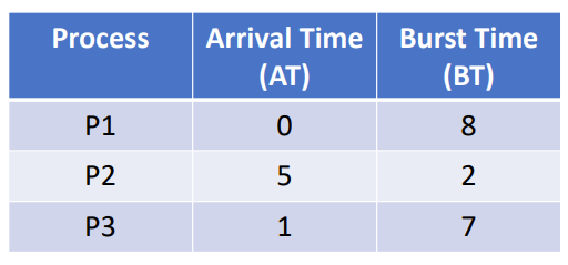
Given a for this system, calculate the:
- Completion Time
- Turn Around Time
- Waiting Time For the following table using round robin scheduling:
Example
At our only process that has arrived is P1, so we run P1 for 3 At P3 arrives, this means the queue is currently P3 At P1 is taken off the CPU, and placed at the end of the queue, (P1 has 5 left) Queue = P3,P1 So now we run P3 for 3 At P2 arrives, our Queue = P1, P2 At P3 is taken off the CPU, and placed at the end of the queue (P3 has 4 left) Queue = P1,P2,P3 P1 is now run for 3 At P1 is taken off the CPU, and placed at the end of the queue, (P1 has 2 left) Queue = P2,P3,P1 P2 is now run, however the remaining time, 2 is less than so we only run for 2 At P2 is finished, and therefore not placed back on the queue Queue = P3,P1 P3 is now run for 3 At P3 is taken off the CPU, and placed at the end of the queue (P3 has 1 left) Queue = P1,P3 P1 is now run, however the remaining time, 2 is less than so we only run for 2 At P1 is finished, and therefore not placed back on the queue Queue = P3 P3 is now run, however the remaining time, 1 is less than so we only run for 1 At P3 is finished, and therefore not placed back on the queue
Therefore we can now create the following.
Shortest Remaining Time First (SRTF)
Algorithm:
- Pre-emptive version of SJF
- Processes are added to a queue, ordered by remaining CPU burst time
- Scheduler is also called when new processes arrive
- Picks the first process in the queue and executes it
- If multiple processes have the same CPU burst time, use FCFS among them Details:
- Fairly simple to implement
- Provable minimum average wait time
Earliest Deadline First (EDF)
Algorithm:
- Each task that arrives has a known deadline
- Start the task with the earliest deadline
- If a new task arrives with an earlier deadline, it skips the queue, and the other task is taken off the CPU Details:
- Optimizes mitigation of maximum lateness
- Allows for new tasks to arrive during the process unlike EDD
Least Laxity (LL)
Algorithm:
- Calculate the time to the deadline minus the remaining execution time for each task. Queue the task with the smallest value
- Each time step recalculate this, if a new task has a lower value, schedule it instead. Details:
- Tries hardest to make sure every task gets finished before the deadline
- In a real system, there is overhead in switching, and certain cases can cause flip flopping between each task every time step (i.e. two identical tasks). Which causes less effective scheduling
Extra Algorithms
Rate Monotonic Scheduling (RMS)
Assumptions:
- Tasks are periodic
- Tasks do not interact
- Single CPU
- Devices are not shared
- No interrupts
Algorithm: Tasks are given priority according to their period, with the shortest period executed first
Pros and Cons:
Pros:
- Easy to implement
- Stable
- Simple to understand Cons:
- Less CPU utilization
- Only can deal with independent tasks
- Unrealistic assumptions for many systems
Determining if Scheduling is Possible Using RMS
Typically for a task like this in a real time system you will be given a bunch of tasks as well as their Execution Time (C), Deadline (D) and their Task Period (T)
We can determine whether a task can be scheduled using two helper values: (Utilization Upper Bound) and (Total Task Utilization) These are defined as such: and Where n is the number of tasks. Finally with these two values, if
- then the tasks can be scheduled
- then the tasks can’t be scheduled
- then we can not tell if the tasks can be scheduled or not.
Abstract
Can the following 3 tasks be scheduled?
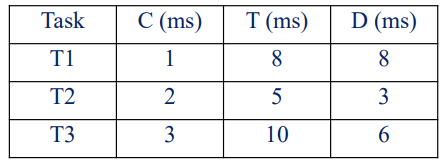
Example
so we can not tell if the tasks can be scheduled or not
Concurrency vs Parallelism
Parallelism
Multiple tasks (threads/processes) execute at the same time. Requires multiple execution units (CPUs, CPU cores, CPU vCores, etc)
Concurrency
Multiple tasks make progress over time. Time-sharing system.
Threads
Can be thought of as a process in a process. The process has its own registers, stack, code in memory etc. A multithreaded process is a process where multiple functions can be executed at the same time.
Race Conditions
A race condition occurs where the final output of a series of parallel or concurrent processes depend on the timing of their scheduling.
Consider two processes PA and PB communicating via shared memory.
Assume shared memory consists of a single integer X = 20
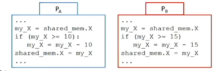 Outcomes:
- PA executes fully before PB:
- PA’s check for X >= 10 succeeds
- X = 10
- PB’s check for X >= 15 fails
- PB executes fully before PA:
- PB’s check for X >= 15 succeeds
- X = 5
- PA’s check for X >= 10 fails
Therefore our solution is to introduce a:
Critical Section:
A critical section is a section of code where a process touches shared resources (shared memory, common variables, shared database, shared file, etc)
Goal: no two processes in their critical section at the same time.
We can see the critical section in from earlier, this can be amended to be as such:
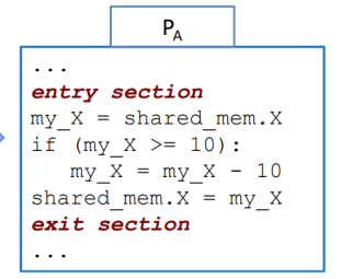
Essentially, when we enter a section, we lock it with something like a Mutex (Mutual Exclusion), which essentially is like a key that locks a section of code, or memory, until it is done. This approach prevents race conditions.
There are disadvantages to this approach, but they aren’t relevant to this course.
State Diagram
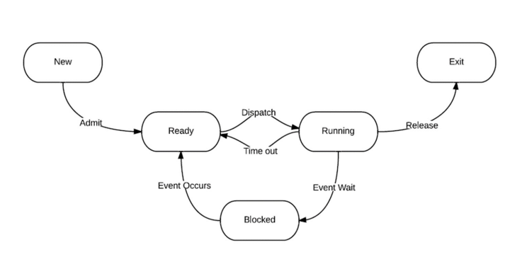 You’ll get marks for memorizing this.
Interrupts can be caused by:
- Scheduling
- Interrupts
- Requests
Each PCB/TCB can contain:
- Process ID
- Process State
- Priority
- Stored Registers
- User Information
Final Note:
As always if you spot a mistake contact: @arsenxc on discord