Simulation of Engineering System Block 3 Cheat Sheet

Abstract:

Block 3, based on the materials of Tutorial 3 (2023), typically is the content used for questions 3 and 4 of Simulation of Engineering Systems, so given that the exam is a choose 2 of 4 style exam, you should hopefully be able to pass with 100% from this material alone

That being said, please don’t rely only on this resource, I’m not liable for them putting only one question on this block in the exam.

If this document kicks about long enough it also may be out of date.

Numerical/Graphical Integration:

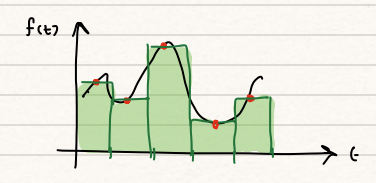
Midpoint Rule:

$${\int }_{t_0}^{t}f(t)dt\approx \sum _{i=1}^n(t_i-t_{i-1})(f(\frac{t_i+t_{i-1}}{2}))$$

Abstract

The response shown in Figure 2 is obtained from the following state equation $\dot{x}=f(t)=2\cos 3t+3\cos 2t$ By using a partition size of 0.5, calculate the values for state x by integrating the curve shown in Figure 2 at each time interval using the Midpoint Rule (from 0-2.5s)

Example

$t$	$0$	$0.25$	$0.5$	$0.75$	$1.0$	$1.25$	$1.5$	$1.75$	$2.0$	$2.25$	$2.5$
$f(t)$	$5$	$4.10$	$1.76$	$-1.04$	$-3.23$	$-4.04$	$-3.39$	$-1.79$	$-0.04$	$1.15$	$1.54$
$
\begin{align}
I_0 &= \int^{0.5}_0 f(t)dt \approx (t_1-t_0)(f(\frac{t_1+t_0}{2})) = (0.5-0)(4.10) = 2.05\
I_1 &= \int^{1.0}_{0.5} f(t)dt \approx (t_2-t_1)(f(\frac{t_2+t_1}{2})) = (1.0-0.5)(-1.04) = -0.52 \
I_2 &= \int^{1.5}_{1.0} f(t)dt \approx (t_3-t_2)(f(\frac{t_3+t_2}{2})) = (1.5-1.0)(-4.04)=-2.02\
I_3 &= \int^{2.0}_{1.5} f(t)dt \approx (t_4-t_3)(f(\frac{t_4+t_3}{2})) = (2.0-1.5)(-1.79) = -0.90 \
I_4 &= \int^{2.5}_{2.0} f(t)dt \approx (t_5-t_4)(f(\frac{t_5+t_4}{2})) = (2.5-2.0)(1.15) = 0.58\
\end{align}
$
Therefore:
$
\begin{align}
t_1&=0.5s, x_1 = x_0+I_0 = 0 + 2.05 = 2.05\
t_2&=1.0s, x_2 = x_1+I_1 = 2.05 + (-0.52) = 1.53\
t_3&=1.5s, x_3 = x_2+I_2 = 1.53 + (-2.02) = -0.49\
t_4&=2.0s, x_4 = x_3+I_3 = -0.49 + (-0.90) = -1.39\
t_5&=2.5s, x_5 = x_4+I_4 = -1.39+0.58 = -0.81\
\end{align}
$
So we deduce that
$
\int^{2.5}_0 2\cos3t + 3\cos2t \approx -0.81
$

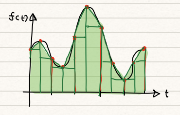
Simpson’s Rule:

$${\int }_{t_0}^{t}f(t)dt\approx \frac{1}{6}\sum _{i=1}^n(t_i-t_{i-1})(f(t_{i-1})+4f(\frac{t_i-t_{i-1}}{2})+f(t_i))$$

Abstract

The response shown in Figure 2 is obtained from the following state equation $\dot{x}=f(t)=2\cos 3t+3\cos 2t$ By using a partition size of 0.5, calculate the values for state x by integrating the curve shown in Figure 2 at each time interval using Simpson’s Rule (from 0-2.5s)

Example

$t$	$0$	$0.25$	$0.5$	$0.75$	$1.0$	$1.25$	$1.5$	$1.75$	$2.0$	$2.25$	$2.5$
$f(t)$	$5$	$4.10$	$1.76$	$-1.04$	$-3.23$	$-4.04$	$-3.39$	$-1.79$	$-0.04$	$1.15$	$1.54$
$
\begin{align}
I_0 &= \int^{0.5}_0 f(t)dt \approx \frac{1}{6}(t_1-t_0)(f(t_0)+4f(\frac{t_1+t_0}{2})+f(t_1)) = \frac{1}{6}(0.5-0)(23.16) = 1.93\
I_1 &= \int^{1.0}_{0.5} f(t)dt \approx \frac{1}{6}(t_2-t_1)(f(t_1)+4f(\frac{t_2+t_1}{2})+f(t_2)) = \frac{1}{6}(1.0-0.5)(-5.63) = -0.47 \
I_2 &= \int^{1.5}_{1.0} f(t)dt \approx \frac{1}{6}(t_3-t_2)(f(t_2)+4f(\frac{t_3+t_2}{2})+f(t_3)) = \frac{1}{6}(1.5-1.0)(-22.78)=-1.90\
I_3 &= \int^{2.0}_{1.5} f(t)dt \approx \frac{1}{6}(t_4-t_3)(f(t_3)+4f(\frac{t_4+t_3}{2})+f(t_4)) =\frac{1}{6} (2.0-1.5)(-10.59) = -0.88 \
I_4 &= \int^{2.5}_{2.0} f(t)dt \approx \frac{1}{6}(t_5-t_4)(f(t_4)+4f(\frac{t_5+t_4}{2})+f(t_5)) = \frac{1}{6}(2.5-2.0)(6.1) = 0.51\
\end{align}
$
Therefore:
$
\begin{align}
t_1&=0.5s, x_1 = x_0+I_0 = 0 + 1.93 = 2.05\
t_2&=1.0s, x_2 = x_1+I_1 = 1.93 + (-0.47) = 1.46\
t_3&=1.5s, x_3 = x_2+I_2 = 1.46 + (-1.90) = -0.44\
t_4&=2.0s, x_4 = x_3+I_3 = -0.44 + (-0.88) = -1.32\
t_5&=2.5s, x_5 = x_4+I_4 = -1.32 + 0.51 = -0.81\
\end{align}
$
So we deduce that
$
\int^{2.5}_0 2\cos3t + 3\cos2t \approx -0.81
$

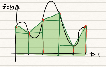
Trapezoid Rule:

$${\int }_{t_0}^{t}f(t)dt\approx \frac{1}{2}\sum _{i=1}^n(t_i-t_{i-1})(f(t_i)+f(t_{i-1}))$$

Abstract

The response shown in Figure 2 is obtained from the following state equation $\dot{x}=f(t)=2\cos 3t+3\cos 2t$ By using a partition size of 0.5, calculate the values for state x by integrating the curve shown in Figure 2 at each time interval using the Trapezoid Rule (from 0-2.5s)

Example

$t$	$0$	$0.25$	$0.5$	$0.75$	$1.0$	$1.25$	$1.5$	$1.75$	$2.0$	$2.25$	$2.5$
$f(t)$	$5$	$4.10$	$1.76$	$-1.04$	$-3.23$	$-4.04$	$-3.39$	$-1.79$	$-0.04$	$1.15$	$1.54$
$
\begin{align}
I_0 &= \int^{0.5}_0 f(t)dt \approx \frac{1}{2}(t_1-t_0)(f(t_1)+f(t_0)) = \frac{1}{2}(0.5-0)(6.76) = 1.69\
I_1 &= \int^{1.0}_{0.5} f(t)dt \approx \frac{1}{2}(t_2-t_1)(f(t_2)+f(t_1)) = \frac{1}{2}(1.0-0.5)(-1.47) = -0.37 \
I_2 &= \int^{1.5}_{1.0} f(t)dt \approx \frac{1}{2}(t_3-t_2)(f(t_3)+f(t_2)) = \frac{1}{2}(1.5-1.0)(-6.62)=-1.66\
I_3 &= \int^{2.0}_{1.5} f(t)dt \approx \frac{1}{2}(t_4-t_3)(f(t_4)+f(t_3)) = \frac{1}{2}(2.0-1.5)(-3.43) = -0.86 \
I_4 &= \int^{2.5}_{2.0} f(t)dt \approx \frac{1}{2}(t_5-t_4)(f(t_5)+f(t_4)) = \frac{1}{2}(2.5-2.0)(1.50) = 0.38\
\end{align}
$
Therefore:
$
\begin{align}
t_1&=0.5s, x_1 = x_0+I_0 = 0 + 1.69 = 1.69\
t_2&=1.0s, x_2 = x_1+I_1 = 1.69 + (-0.37) = 1.32\
t_3&=1.5s, x_3 = x_2+I_2 = 1.32 + (-1.66) = -0.34\
t_4&=2.0s, x_4 = x_3+I_3 = -0.34 + (-0.86) = -1.2\
t_5&=2.5s, x_5 = x_4+I_4 = -1.2 + 0.38 = -0.82\
\end{align}
$
So we deduce that:
$
\int^{2.5}_0 2\cos3t + 3\cos2t \approx -0.82
$

Errors:

Absolute Error:

$$e_A=|\mathbf{real}-\mathbf{estimate}|$$

Abstract

Find the absolute error of the value of the integral of: $\dot{x}=f(t)=2\cos 3t+3\cos 2t$ From 0 to 2 seconds Comparing the value estimated by the Trapezoid Rule and Simpson’s Rule, against a calculated value for the integral

Example

\begin{align} x &= \int^{2.0}_0 \dot{x}dx = [\frac{2}{3}\sin3t + \frac{3}{2}\sin2t]^{2.0}_0 \\ x &= \frac{2}{3}\sin(6.0)+\frac{3}{2}\sin(4.0) = -1.32 \end{align} \begin{align} \textbf{Simpson : } e_A &= |-1.32 -(-1.32)| = 0.0 \\ \textbf{Trapezoid : } e_A &= |-1.32 - (-1.2)| = 0.12 \end{align}

Relative Error:

$$e_R=\frac{e_A}{|\text{real}|}$$

Abstract

From the previous question calculate the relative error for both the Trapezoid and Simpson’s Rule

Example

\begin{align} \textbf{Simpson : }e_R &= \frac{0.0}{|-1.32|} = 0 \\ \textbf{Trapezoid : }e_R &= \frac{0.12}{|-1.32|} = 0.091 \end{align}

Newton’s Interpolation

$$\begin{array}{rl}•& \text{ Constant}\\ & P_0(x)=b\\ •& \text{ Linear}\\ & P_1(x)=P_0(x)+c_1(x-x_1)\\ •& \text{ Quadratic}\\ & P_2(x)=P_1(x)+c_2(x-x_1)(x-x_2)\\ •& \text{ Nth Order}\\ & P_n(x)=P_{n-1}(x)+c_n(x-x_1)(x-x_2)(...)(x-x_{n-1})(x-x_n)\end{array}$$

Abstract

From the following set of data calculate the interpolated $P_3(x)$

$x$	$1$	$\frac{3}{2}$	$0$	$2$
$f(x)$	$3$	$\frac{13}{4}$	$3$	$\frac{5}{3}$

Example

\begin{align} •& \textbf{ Constant} \\ &P_0(x) = 3 \\ & \\ •& \textbf{ Linear} \\ &P_1(x) = P_0(x) + c_1(x-x_1) \\ & = 3 + c_1(x-1)\\ &\frac{13}{4} = 3 +c_1(\frac{3}{2}-1) \\ &\therefore c_1 = \frac{1}{2} \\ &\therefore P_1(x) = 3 + \frac{1}{2}(x-1) = \frac{5}{2} + \frac{1}{2}x \\ & \\ \end{align} \begin{align} •& \textbf{ Quadratic} \\ &P_2(x) = P_1(x) + c_2(x-x_1)(x-x_2) \\ & = \frac{5}{2} + \frac{1}{2}x + c_2(x-1)(x-\frac{3}{2})\\ & 3 =\frac{5}{2} + c_2(0-1)(0-\frac{3}{2}) \\ &\therefore c_2 = \frac{1}{3} \\ &\therefore P_2(x) = \frac{5}{2} + \frac{1}{2}x + \frac{1}{3}(x-1)(x-\frac{3}{2}) \\ & \\ \end{align} \begin{align} •& \textbf{ Cubic} \\ &P_3(x) = P_2(x) + c_3(x-x_1)(x-x_2)(x-x_3) \\ & = \frac{5}{2} + \frac{1}{2}x + \frac{1}{3}(x-1)(x-\frac{3}{2}) +c_3(x-1)(x-\frac{3}{2})x\\ & \frac{5}{3} = \frac{5}{2} + \frac{1}{2}*2 + \frac{1}{3}(2-1)(2-\frac{3}{2}) + c_3(2-1)(2-\frac{3}{2})2 \\ &\therefore c_3 = -2 \\ &\therefore P_3(x) = \frac{5}{2} + \frac{1}{2}x + \frac{1}{3}(x-1)(x-\frac{3}{2}) -2 (x-1)(x-\frac{3}{2})x \\ & \\ \end{align} So our final answer is $P_3(x)=\frac{5}{2}+\frac{1}{2}x+\frac{1}{3}(x-1)(x-\frac{3}{2})-2(x-1)(x-\frac{3}{2})x$

Newton Divided Difference:

$x$	$F[]$	$F[,]$	$F[,,]$	$F[,,,]$
$x_1$	$F[x_1]$
$x_2$	$F[x_2]$	$F[x_1,x_2]$ = $\frac{F[x_2]-F[x_1]}{x_2-x_1}$
$x_3$	$F[x_3]$	$F[x_2,x_3]$ = $\frac{F[x_3]-F[x_2]}{x_3-x_2}$	$F[x_1,x_2,x_3]$ = $\frac{F[x_2,x_3]-F[x_1,x_2]}{x_3-x_1}$
$x_3$	$F[x_4]$	$F[x_3,x_4]$ = $\frac{F[x_4]-F[x_3]}{x_4-x_3}$	$F[x_2,x_3,x_4]$ = $\frac{F[x_3,x_4]-F[x_2,x_3]}{x_4-x_2}$	$F[x_1,x_2,x_3,x_4]$ = $\frac{F[x_2,x_3,x_4]-F[x_1,x_2,x_3]}{x_4-x_1}$

Which we can then convert to:

$a_n$	$F[]$
$a_0$	$F[x_1]$
$a_1$	$F[x_1,x_2]$
$a_2$	$F[x_1,x_2,x_3]$
$a_3$	$F[x_1,x_2,x_3,x_4]$

Standard Form:

$$P_3(x)=a_0+a_1(x-x_1)+a_2(x-x_1)(x-x_2)+a_3(x-x_1)(x-x_2)(x-x_3)$$

Nested Form:

$$P_3(x)=a_0+(x-x_1)(a_1+(x-x_2)(a_2+a_3(x-x_3)))$$

Abstract

For the following table derive the Newton’s Divided Difference

$x$	$1$	$\frac{3}{2}$	$0$	$2$
$f(x)$	$3$	$\frac{13}{4}$	$3$	$\frac{5}{3}$

Example

$x$	f[]	f[,]	f[,,]	f[,,,]
1	3
$\frac{3}{2}$	$\frac{13}{4}$	$F[x_1,x_2]$ = $\frac{F[x_2]-F[x_1]}{x_2-x_1}=\frac{13/4-3}{3/2-1}=1/2$
0	3	$F[x_2,x_3]$ = $\frac{F[x_3]-F[x_2]}{x_3-x_2}=\frac{3-13/4}{0-3/2}=1/6$	$F[x_1,x_2,x_3]$ = $\frac{F[x_2,x_3]-F[x_1,x_2]}{x_3-x_1}=\frac{1/6-1/2}{0-1}=1/3$
2	$\frac{5}{3}$	$F[x_3,x_4]$ = $\frac{F[x_4]-F[x_3]}{x_4-x_3}=\frac{5/3-3}{2-0}=2/3$	$F[x_2,x_3,x_4]$ = $\frac{F[x_3,x_4]-F[x_2,x_3]}{x_4-x_2}=\frac{2/3-1/6}{2-3/2}=-5/3$	$F[x_1,x_2,x_3,x_4]$ = $\frac{F[x_2,x_3,x_4]-F[x_1,x_2,x_3]}{x_4-x_1}=\frac{-5/3-1/3}{2-1}=-2$
$
\begin{align}
a_0 = 3, a_1 = \frac{1}{2}, a_2 = \frac{1}{3}, a_3=-2
\end{align}
$
$
P_3(x) = 3 + \frac{1}{2}(x-1) + \frac{1}{3}(x-1)(x-\frac{3}{2}) -2(x-1)(x-\frac{3}{2})(x)
$
$
P_3(x) = 3 + (x-1)(\frac{1}{2} + (x-\frac{3}{2})(\frac{1}{3}-2x) )
$

Splines:

Linear Splines:

$$S_i(x)=\frac{f_{i+1}-f_i}{x_{i+1}-x_i}x+b_i$$

To note: $b_i$ is derived from the fact $S_i(x)$ should equal $f(x)$ at $S_i(x_i)$

Abstract

Interpolate these data points using Linear Splines:

$t$	$-150$	$-85$	$57$	$113$	$167$
$g(t)$	$-0.866$	$0.087$	$0.545$	$-0.391$	$-0.974$

Example

\begin{align} \textbf{Spline 1}&: S_1(t) = a_1t + b_1 \\ \textbf{Slope } a_1 &= \frac{0.087 - (-0.866)}{-85-(-150)} = \frac{0.953}{65} = 0.0147 \\ \text{at } t=-85& \text{ , } S_1(-85)=0.087 \\ \therefore \text{ }& 0.0147*-85+b_1 = 0.087 \\ & b_1 = 1.3365 \\ \therefore \text{ }&S_1(t) = 0.0147t + 1.3365 \\ &\\ &\\ \end{align} \begin{align} \textbf{Spline 2}&: S_2(t) = a_2t + b_2 \\ \textbf{Slope } a_2 &= \frac{0.545 - 0.087}{57-(-85)} = \frac{0.458}{142} = 0.0032 \\ \text{at } t=57& \text{ , } S_2(57)=0.545 \\ \therefore \text{ }& 0.0032*57+b_2 = 0.545 \\ & b_2 = 0.3626 \\ \therefore \text{ }&S_2(t) = 0.0032t + 0.3626 \\ &\\ &\\ \end{align} \begin{align} \textbf{Spline 3}&: S_3(t) = a_3t+ b_3 \\ \textbf{Slope } a_3 &= \frac{-0.391 - 0.545}{113-57} = \frac{-0.936}{56} = -0.0167 \\ \text{at } t=113& \text{ , } S_3(113)=-0.391 \\ \therefore \text{ }& -0.0167*113+b_3 = -0.391 \\ & b_3 = 1.4961 \\ \therefore \text{ }&S_3(t) = -0.0167t + 1.4961 \\ &\\ &\\ \end{align} \begin{align} \textbf{Spline 4}&: S_4(t) = a_4t+ b_4 \\ \textbf{Slope } a_4 &= \frac{-0.974 - (-0.391)}{167-113} = \frac{-0.583}{54} = -0.0108 \\ \text{at } t=167& \text{ , } S_4(167)=-0.974 \\ \therefore \text{ }& -0.0108*167+b_4 = -0.974 \\ & b_4 = 0.8296 \\ \therefore \text{ }&S_4(t) = -0.0108t + 0.8296 \\ &\\ &\\ \end{align} $S(t)=\{\begin{array}{ll}{S}_1(t)=0.0147t+1.3365& \text{if }-150\le x\le -85\\ S_2(t)=0.0032t+0.3626& \text{if }-85\le x\le 57\\ S_3(t)=-0.0167t+1.4961& \text{if }57\le x\le 113\\ S_4(t)=-0.0108t+0.8296& \text{if }113\le x\le 167\end{array}$

Quadratic Splines:

$$S_i(x)=\frac{z_{i+1}-z_i}{2(x_{i+1}-x_i)}(x-x_i{)}^2+z_i(x-x_i)+f(x_i)$$

Where:

$$z_{i+1}=-z_i+2(\frac{y_{i+1}-y_i}{x_{i+1}-x_i})$$

Abstract

Interpolate these data points using Quadratic Splines:

$t$	$-150$	$-85$	$57$	$113$	$167$
$g(t)$	$-0.866$	$0.087$	$0.545$	$-0.391$	$-0.974$

Example

\begin{align} \textbf{Slope}&\textbf{ Values at Knots:} \\ z_1 &= 0 \text{ (Assumed)} \\ z_2 &= -z_1 + 2(\frac{g_2-g_1}{t_2-t_1}) = -0 + 2(\frac{0.087 - (-0.866)}{-85-(-150)}) = 0.0293 \\ z_3 &= -z_2 + 2(\frac{g_3-g_2}{t_3-t_2}) = -0.0293 + 2(\frac{0.545 - 0.087}{57-(-85)}) = -0.0228 \\ z_4 &= -z_3 + 2(\frac{g_4-g_3}{t_4-t_3}) = 0.0228 + 2(\frac{-0.391 - 0.545}{113-57}) = -0.0106 \\ z_5 &= -z_4 + 2(\frac{g_5-g_4}{t_5-t_4}) = 0.0106 + 2(\frac{-0.974 - (-0.391)}{167-113}) = -0.0110 \\ &\\ &\\ \end{align} \begin{align} S_1(t) &= \frac{z_2-z_1}{2(t_2-t_1)}(t-t_1)^2 + z_1(t-t_1) +g_1 \\ S_1(t) &= \frac{0.0293 - 0}{2(-85-(-150))}(t+150)^2 + 0(t+150) - 0.866 \\ S_1(t) &= 2.254*10^{-4}(t+150)^2-0.866 \\ &\\ &\\ \end{align} \begin{align} S_2(t) &= \frac{z_3-z_2}{2(t_3-t_2)}(t-t_2)^2 + z_2(t-t_2) +g_2 \\ S_2(t) &= \frac{-0.0228-0.0293}{2(57-(-85))}(t+85)^2 + 0.0293(t+85) + 0.087 \\ S_2(t) &= -1.838*10^{-4}(t+85)^2+0.0293(t+85)+0.087 \\ &\\ &\\ \end{align} \begin{align} S_3(t) &= \frac{z_4-z_3}{2(t_4-t_3)}(t-t_3)^2 + z_3(t-t_3) +g_3 \\ S_3(t) &= \frac{-0.0106-(-0.0228)}{2(113-57)}(t-57)^2 - 0.0228(t-57) + 0.545 \\ S_3(t) &= 1.089*10^{-4}(t-57)^2-0.0228(t-57)+0.545 \\ &\\ &\\ \end{align} \begin{align} S_4(t) &= \frac{z_5-z_4}{2(t_5-t_4)}(t-t_4)^2 + z_4(t-t_4) +g_4 \\ S_4(t) &= \frac{-0.0110-(-0.0106)}{2(167-113)}(t-113)^2 - 0.0106(t-113) - 0.391 \\ S_4(t) &= -0.037*10^{-4}(t-113)^2-0.0106(t-113)-0.391 \\ &\\ &\\ \end{align} $S(t)=\{\begin{array}{ll}{S}_1(t)=2.254\ast 10^{-4}(t+150{)}^2-0.866& \text{if }-150\le x\le -85\\ S_2(t)=-1.838\ast 10^{-4}(t+85{)}^2+0.0293(t+85)+0.087& \text{if }-85\le x\le 57\\ S_3(t)=1.089\ast 10^{-4}(t-57{)}^2-0.0228(t-57)+0.545& \text{if }57\le x\le 113\\ S_4(t)=-0.037\ast 10^{-4}(t-113{)}^2-0.0106(t-113)-0.391& \text{if }113\le x\le 167\end{array}$

Extra Note:

If something on this document is wrong, or you want to add something, or want the original markdown I made this in contact me via:

• Discord : @arsenxc
• Github : StefVuck

Gist: https://gist.github.com/StefVuck/1006355703e01c008aa0e7d4a386f424