DSP Tutorial

Question 1:

Question

Sketch the spectrum of a 1kHz Sine-wave with an amplitude of 2 sampled at 10kHz as an analogue plot $X(F)$ and as it sampled counterpart $X(k)$. Include the negative frequency alias (aka “mirror frequencies”) in your plot. Label it appropiately

\begin{document}
  \begin{tikzpicture}[domain=0:6.28]
  	\draw (0,2) node[left] {2};
  	\draw[dashed,gray] (0,2) -- (6.28,2);
  	\draw (0,-2) node[left] {-2};
  	\draw[dashed,gray] (0,-2) -- (6.28,-2);
    \draw[->] (-0.2,0) -- (8.28,0) node[right] {$x$};
    \draw[->] (0,-2.2) -- (0,2.2) node[above] {$f(x)$};
    \draw[color=orange]   plot (\x,{2*sin(\x r)})    node[above] {$f(x) = \sin x$};
  \end{tikzpicture}
\end{document}

\begin{document}
\begin{tikzpicture}
\draw[->] (-5,0) -- (5,0) node[right] {f (kHz)};
\draw[->] (0,0) -- (0,3) node[above] {X(f)};
\draw[thick] (1,0) -- (1,2);
\draw[thick] (-1,0) -- (-1,2);
\draw (0,0) node[below] {0};
\draw (1,0) node[below] {1};
\draw (-1,0) node[below] {-1};
 
\end{tikzpicture}
\end{document}

\begin{document}
\begin{tikzpicture}
\draw[->] (0,0) -- (16,0) node[right] {K};
\draw[->] (0,0) -- (0,3) node[above] {X(f)};
\draw[thick] (1,0) -- (1,2);
\draw[thick] (9,0) -- (9,2);
\draw[thick] (11,0) -- (11,2);
\draw (0,0) node[below] {0};
\draw (1,0) node[below] {N/10};
\draw (5,0) node[below] {5N/10};
\draw (9,0) node[below] {9N/10};
\draw (11,0) node[below] {11N/10};
\draw (19,0) node[below] {19N/10};
\draw[thick] (16,1) node[scale=3] {...};
\draw (10,0) node[below] {Fs};
\draw (15,0) node[below] {15N/10};
 
\draw[dashed,gray] (5,0) -- (5,2.5);
\draw[dashed,gray] (10,0) -- (10,2.5);
\draw[dashed,gray] (15,0) -- (15,2.5);
\end{tikzpicture}
\end{document}

Question 2:

Question

You send the sine wave through a limiter which limits the sine wave at 0.5. Sketch the analogue and digital spectrums again

\begin{document}
  \begin{tikzpicture}[domain=0:6.28]
	\draw (0,0.5) node[left] {0.5};
	\draw[dashed,gray] (0,0.5) -- (6.28,0.5);
	\draw (0,-0.5) node[left] {-0.5};
	\draw[dashed,gray] (0,-0.5) -- (6.28,-0.5);
    \draw[->] (-0.2,0) -- (8.28,0) node[right] {$x$};
    \draw[->] (0,-1.2) -- (0,1.2) node[above] {$f(x)$};
    \draw[color=orange]   plot (\x,{max(-0.5, min(0.5, 2*sin(\x r)))}) node[above] {$f(x) = 2\sin x$};
  \end{tikzpicture}
\end{document}

Digital:

\begin{document}
\begin{tikzpicture}
\draw[->] (0,0) -- (16,0) node[right] {K};
\draw[->] (0,0) -- (0,3) node[above] {X(f)};
\draw[thick] (1,0) -- (1,2);
\draw[thick] (3,0) -- (3,1);
\draw[thick] (5,0) -- (5,0.5);
\draw[thick] (7,0) -- (7,1);
\draw[thick] (9,0) -- (9,2);
\draw[thick] (11,0) -- (11,2);
\draw[thick] (13,0) -- (13,1);
\draw[thick] (15,0) -- (15,0.5);
\draw (0,2.15) node[left] {0.5};
\draw[thick] (-0.25,2) -- (0.25,2);
\draw[dashed,gray] (0,2) -- (16,2);
\draw (0,0) node[below] {0};
\draw (1,0) node[below] {N/10};
\draw (3,0) node[below] {3N/10};
\draw (5,0) node[below] {5N/10};
\draw (7,0) node[below] {7N/10};
\draw (9,0) node[below] {9N/10};
\draw (11,0) node[below] {11N/10};
\draw (13,0) node[below] {13N/10};
\draw (15,0) node[below] {15N/10};
\draw[thick] (16,1) node[scale=3] {...};
\draw (10,0) node[below] {Fs};
 
\draw[dashed,gray] (10,0) -- (10,2.5);
\end{tikzpicture}
\end{document}

Analog:

\begin{document}
\begin{tikzpicture}
\draw[->] (-8,0) -- (8,0) node[right] {f (kHz)};
\draw[->] (0,0) -- (0,3) node[above] {X(f)};
\draw[thick] (1,0) -- (1,1.8);
\draw[thick] (3,0) -- (3,1);
\draw[thick] (5,0) -- (5,0.5);
\draw[thick] (7,0) -- (7,0.25);
\draw[thick] (-1,0) -- (-1,1.8);
\draw[thick] (-3,0) -- (-3,1);
\draw[thick] (-5,0) -- (-5,0.5);
\draw[thick] (-7,0) -- (-7,0.25);
\draw (0,2.15) node[left] {0.25};
\draw[thick] (-0.25,2) -- (0.25,2);
\draw (0,0) node[below] {0};
\draw (1,0) node[below] {1};
\draw (3,0) node[below] {3};
\draw (5,0) node[below] {5};
\draw (7,0) node[below] {7};
\draw (-1,0) node[below] {-1};
\draw (-3,0) node[below] {-3};
\draw (-5,0) node[below] {-5};
\draw (-7,0) node[below] {-7};
 
\draw[dashed,gray] (-8,2) -- (8,2);
\end{tikzpicture}
\end{document}

Only the odd harmonics appear as the signal is symmetrical The main peaks don’t actually reach 0.25, as they all add up to it together

Question 3

Question

A guitar amp has usually two controls: “drive” and “volume” where drive controls the gain before the signal enters the non-linearity and volume after it. Which one is important to create a perceptually loud output

Has to be before non-linearity as that is the component that creates the relative loudness, you can’t affect the perceived loudness after this point, only the actual volume.

The way to imagine it, is that the non linearity will make the maximum usage of the total energy by making the “important” sections take up more of the total energy while reducing the amount used by a “non-important” components

Question 4

Question

The original Zoom H4 is a great recorder for ambient sounds but uses a switching power supply for its mics so that there is a faint 8kHz tone in every recording. The sampling rate is 48khz. Describe how to elimiate this tone with the help of the Fourier Transform decisign an efficient coding approach in Python. Write down the commands.

def remove_8k(signal):
	f_sig = np.fft.ftt(signal)
	target_idx = N * (8/48)
	bounds = N * (50/48000)
	
	f_sig[(target_idx - bounds) : (target_idx + bounds)] = 0
	f_sig[-(target_idx + bounds) : -(target_idx - bounds)] = 0
	
	signal = np.fft.ifft(f_sig)
	return signal

Tutorial 2

Question 1

Question

Sketch the frequency response of a digital bandstop filter and perform an inverse Fourier Transform to obtain the impulse response

\begin{document}
\begin{tikzpicture}
    % Axes
    \draw[->] (-8,0) -- (8,0) node[right] {Frequency (Hz)};
    \draw[->] (0,0) -- (0,4) node[above] {Magnitude};
 
    % Positive Frequency Response
    \draw[thick, blue, smooth] 
        (0,3) -- (3,3) -- (3,0.5) -- (5,0.5) -- (5,3) -- (7.5,3);
 
    % Negative Frequency Response (mirrored)
    \draw[thick, blue, smooth] 
        (-0,3) -- (-3,3) -- (-3,0.5) -- (-5,0.5) -- (-5,3) -- (-7.5,3);
 
    % Stopband markers for positive frequencies
    \draw[dashed] (3,0) -- (3,3);
    \draw[dashed] (5,0) -- (5,3);
    \node[below] at (3,0) {$f_{low}$};
    \node[below] at (5,0) {$f_{high}$};
 
    % Stopband markers for negative frequencies
    \draw[dashed] (-3,0) -- (-3,3);
    \draw[dashed] (-5,0) -- (-5,3);
    \node[below] at (-3,0) {$-f_{low}$};
    \node[below] at (-5,0) {$-f_{high}$};
 
    % Text annotations
    \node[above] at (1,3.2) {Passband};
    \node[above] at (4,0.7) {Stopband};
    \node[above] at (6.5,3.2) {Passband};
    \node[above] at (-1,3.2) {Passband};
    \node[above] at (-4,0.7) {Stopband};
    \node[above] at (-6.5,3.2) {Passband};
\end{tikzpicture}
\end{document}
 

But it comes out practically more like:

\begin{document}
\begin{tikzpicture}
    % Axes
    \draw[->] (-8,0) -- (8,0) node[right] {Frequency (Hz)};
    \draw[->] (0,0) -- (0,4) node[above] {Magnitude};
 
    % Positive Frequency Response
    \draw[thick, blue, smooth] 
        (0,3) -- (2,3) -- (3,0.5) -- (5,0.5) -- (6,3) -- (7.5,3);
 
    % Negative Frequency Response (mirrored)
    \draw[thick, blue, smooth] 
        (-0,3) -- (-2,3) -- (-3,0.5) -- (-5,0.5) -- (-6,3) -- (-7.5,3);
 
    % Stopband markers for positive frequencies
    \draw[dashed] (3,0) -- (3,3);
    \draw[dashed] (5,0) -- (5,3);
    \node[below] at (3,0) {$f_{low}$};
    \node[below] at (5,0) {$f_{high}$};
 
    % Stopband markers for negative frequencies
    \draw[dashed] (-3,0) -- (-3,3);
    \draw[dashed] (-5,0) -- (-5,3);
    \node[below] at (-3,0) {$-f_{low}$};
    \node[below] at (-5,0) {$-f_{high}$};
 
    % Text annotations
    \node[above] at (1,3.2) {Passband};
    \node[above] at (4,0.7) {Stopband};
    \node[above] at (6.5,3.2) {Passband};
    \node[above] at (-1,3.2) {Passband};
    \node[above] at (-4,0.7) {Stopband};
    \node[above] at (-6.5,3.2) {Passband};
\end{tikzpicture}
\end{document}
 

Sort of like this:

\begin{document}
\begin{tikzpicture}
    \draw[->] (0,0) -- (3.14,0) node[right] {Samples (n)};
    \draw[->] (0,-1.5) -- (0,1.5) node[above] {Amplitude};
% Draw function
	\draw[blue, smooth, samples=200, domain=0.01:3.14] plot (\x,{sin(\x*6 r))/(\x*6)});
 
    % Annotate
    \node[above] at (4,0.5) {Impulse Response};
\end{tikzpicture}
\end{document}

$$h[n]={\mathcal{F}}^{-1}\{H(e^{j\omega })\}=\frac{1}{2\pi }{\int }_{-\pi }^{\pi }H(e^{j\omega })e^{j\omega n}d\omega$$ $$\begin{array}{rl}h[n]& =\frac{1}{2\pi }\left({\int }_{-\pi }^{-{\omega }_{\text{high}}}{e}^{j\omega n}d\omega +{\int }_{-{\omega }_{\text{low}}}^{{\omega }_{\text{low}}}{e}^{j\omega n}d\omega +{\int }_{{\omega }_{\text{high}}}^{\pi }{e}^{j\omega n}d\omega \right)\\ & =\frac{1}{2\pi }\left({\int }_{-\pi }^{-{\omega }_{\text{high}}}{e}^{j\omega n}d\omega +{\int }_{{\omega }_{\text{high}}}^{\pi }{e}^{j\omega n}d\omega \right)+\frac{1}{2\pi }{\int }_{-{\omega }_{\text{low}}}^{{\omega }_{\text{low}}}{e}^{j\omega n}d\omega .\end{array}$$

For each integral, evaluate

1. For $\int e^{j\omega n}d\omega$: $$\int e^{j\omega n}d\omega =\frac{1}{jn}{e}^{j\omega n}.$$

Using this, we compute each term:

$$\begin{array}{rl}{\int }_{-\pi }^{-{\omega }_{\text{high}}}{e}^{j\omega n}d\omega & =\frac{1}{jn}{\left[e^{j\omega n}\right]}_{-\pi }^{-{\omega }_{\text{high}}}=\frac{1}{jn}\left(e^{-j{\omega }_{\text{high}}n}-e^{-j\pi n}\right),\\ {\int }_{{\omega }_{\text{high}}}^{\pi }{e}^{j\omega n}d\omega & =\frac{1}{jn}{\left[e^{j\omega n}\right]}_{{\omega }_{\text{high}}}^{\pi }=\frac{1}{jn}\left(e^{j\pi n}-e^{j{\omega }_{\text{high}}n}\right),\\ {\int }_{-{\omega }_{\text{low}}}^{{\omega }_{\text{low}}}{e}^{j\omega n}d\omega & =\frac{1}{jn}{\left[e^{j\omega n}\right]}_{-{\omega }_{\text{low}}}^{{\omega }_{\text{low}}}=\frac{1}{jn}\left(e^{j{\omega }_{\text{low}}n}-e^{-j{\omega }_{\text{low}}n}\right).\end{array}$$

Substituting back into the expression for ( h[n] ):

$$\begin{array}{rl}h[n]& =\frac{1}{2\pi }\frac{1}{jn}\left(e^{-j{\omega }_{\text{high}}n}-e^{-j\pi n}+e^{j\pi n}-e^{j{\omega }_{\text{high}}n}\right)\\ & +\frac{1}{2\pi }\frac{1}{jn}\left(e^{j{\omega }_{\text{low}}n}-e^{-j{\omega }_{\text{low}}n}\right).\end{array}$$

$e^{-j{\omega }_{high}n}-e^{j{\omega }_{high}n}=-(e^{j{\omega }_{high}n}-e^{-j{\omega }_{high}n})=-2\sin ({\omega }_{high}n)$ $e^{j{\omega }_{low}n}-e^{-j{\omega }_{low}n}=2\sin ({\omega }_{low}n)$ $e^{j\pi n}-e^{-j\pi n}=2\sin (\pi n),\sin (\pi n)=0,\forall n\in \mathbb{Z}$

$$h[n]=\{\begin{array}{ll}\frac{-1}{\pi n}\sin ({\omega }_{high}n)+\frac{1}{\pi n}\sin ({\omega }_{low}n)=\frac{sin({\omega }_{low}n)-sin({\omega }_{high}n)}{\pi n}& \text{for }n\ne 0\\ \frac{{\omega }_{high}-{\omega }_{low}}{\pi }& \text{for }n=0\end{array}$$

Question 2

Question

You used the bandstop filter to remove 50Hz from your ECG in the lab. What are the challenges when you take the impulse response from 1) when designing a narrow bandstop

When designing a narrow bandstop filter to remove 50 Hz from an ECG signal, the primary challenge is the long impulse response that results from the narrow bandwidth. This increases computational complexity and introduces ringing artifacts, which can distort other components of the ECG signal. High filter orders needed for narrowband filtering can also lead to stability issues. Additionally, precise alignment with the target frequency is required; any inaccuracies in sampling rate or signal quantization can reduce the filter’s effectiveness. These challenges require careful design to maintain signal fidelity while achieving effective noise removal.

Question 3

Question

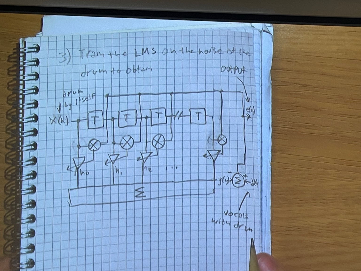
You want to record vocals of a music performance but reight behind the vocal mics is a drum. Explain how to eliminate the drum from the vocals using an LMS filter and two mics.

To eliminate drum sounds from a vocal recording using an adaptive LMS filter, you begin by setting up two microphones in strategic positions. The first microphone, is placed near the vocalist to capture the vocal signal while still allowing some bleed from the drum sound. The second microphone, is positioned closer to the drum source to capture a signal dominated by drum noise with minimal vocal content. These two signals, serve as inputs to the LMS filter.

.

DSP Tutorial 3 (FIR + IIR)

Question 1

Question

As you know, ECG has motion artifacts which are mostly due to the patient moving around. The toy sensors also has an in-built xyz accelerometer and even a magnetometer (compass). How could these 3 or 6 singlas be used to reduce the baseline wander with LMS? Draw a dataflow diagram

Parallel Approach

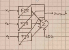
1. Inputs: Multiple motion-related signals ($x_1$, $x_2$, $x_3$)
2. Process: The FIR filters process the motion signals to extract relevant components that correlate with the noise
3. Output Processing: The filtered outputs are summed and subtracted from the raw ECG signal
4. Result: This subtraction yields the clean ECG signal at the output

Cascading Approach

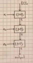
1. Input Processing: Each motion signal ($x_1$, $x_2$, $x_3$) is independently fed into a separate LMS adaptive filter
2. Adaptation: Each LMS filter computes an artifact estimation by minimizing the error between the ECG signal and the artifact correlated with the specific motion signal
3. Combination: The outputs of the individual LMS filters are summed together to estimate the motion artifact
4. Final Output: The estimated artifact is subtracted from the raw ECG to produce the cleaned ECG signal

Question 2

Question

An IIR filter has the transfer function: $H(z)=\frac{1}{1+0.5z^{-1}}$ a) Is it stable? b) write down the impulse response of the filter for 5 samples c) how many multiplication operations are needed for floating point and how many for integer arithmetic?

Stability Analysis

To determine stability:

1. Find poles where: $1+0.5z^{-1}=0$
2. Solving for z:
   • • $z^{-1}=-2$
   • $z=0.5$
3. Result: $|z|\le 1\to 0.5\le 1$ Therefore, as our pole lies in the unit circle, our filter is stable

Impulse Response

For impulse input $x(n)$:

• $x(n)=1$ for $n=0$
• $x(n)=0$ for $n>0$

Difference equation:

$$\begin{array}{rl}H(z)& =\frac{Y(z)}{X(z)}=\frac{1}{1+0.5z^{-1}}\\ X(z)& =Y(z)\ast (1+0.5z^{-1})\\ Y(z)& =X(z)-Y(z)\ast 0.5z^{-1}\\ \therefore y(n)& =x(n)-0.5y(n-1)\end{array}$$

Values for first 5 samples:

1. $x=\delta =1,y(-1)=0,$ $\Rightarrow y(0)=x(0)-0.5y(-1)=1$
2. $x=0,y(0)=1,$ $\Rightarrow y(1)=x(1)-0.5y(0)=-0.5$
3. $x=0,y(1)=-0.5,$ $\Rightarrow y(2)=x(2)-0.5y(1)=0.25$
4. $x=0,y(2)=0.25,$ $\Rightarrow y(3)=x(3)-0.5y(2)=-0.125$
5. $x=0,y(3)=-0.125,$ $\Rightarrow y(4)=x(4)-0.5y(3)=0.0625$

\begin{document}
\begin{tikzpicture}
\draw[->] (-0,0) -- (5,0) node[right] {n};
\draw[->] (0,-3) -- (0,3) node[above] {y(n)};
\draw[thick,red] (0,0) -- (0,2);
\draw[thick,red] (1,0) -- (1,-1);
\draw[thick,red] (2,0) -- (2,0.5);
\draw[thick,red] (3,0) -- (3,-0.25);
\draw[thick,red] (4,0) -- (4,0.125);
\draw (-.25,2) node[left] {1};
\draw (0,-1) node[left] {-0.5};
\draw[dashed,gray] (0,-1) -- (1,-1);
\draw[thick] (-0.125,2) -- (0.125,2);
\end{tikzpicture}
\end{document}

Multiplication Operations Analysis

Question

How many multiplication operations are needed for floating point and how many for efficient integer arithmetic?

Answer

• Floating point: 1 multiplication required
• Efficient integer arithmetic: 0 multiplications (replaced by bit shifts)