IIR Filters

IIR filter stands for Infinite Impulse Response. Such filters have feedback so that signals are processed in a recursive way.

General Form

$$H(z)=\frac{{\Sigma }_{k=0}^r{B}_k{z}^{-k}}{1+{\Sigma }_{l=1}^m{A}_l{z}^{-l}}$$

Where $B_k$ is the FIR coefficients and $A_l$ is the recursive coefficients. Notice how the sign of the recursive coeffs is inverted in the actual implementation of the filter. This is because this $H(z)$ is multiplied with an input signal to obtain the output. The “1” in the denominator actually represents the output of the filter, if the factor is not 1, the output is scaled by that factor.

IIR Filter Design Steps:

(for a second order filter)

1. Choose the cut-off frequency of your digital filter ${\omega }_c$.
2. Calculate the analogue cutoff frequency ${\omega }_c$ → ${\Omega }_c$ with this eq
3. Choose your favourite analogue lowpass filter $H(s)$, for example Butterworth.
4. Replace all $s$ in the analogue transfer function $H(s)$ by $s=\frac{2}{T}\frac{z-1}{z+1}$ to obtain the digital filter $H(z)$
5. Change the transfer function $H(z)$ so that it only contains negative powers of $z(z^{-1},z^{-2},...)$ which can be interpreted as delay lines.
6. Build your IIR filter!

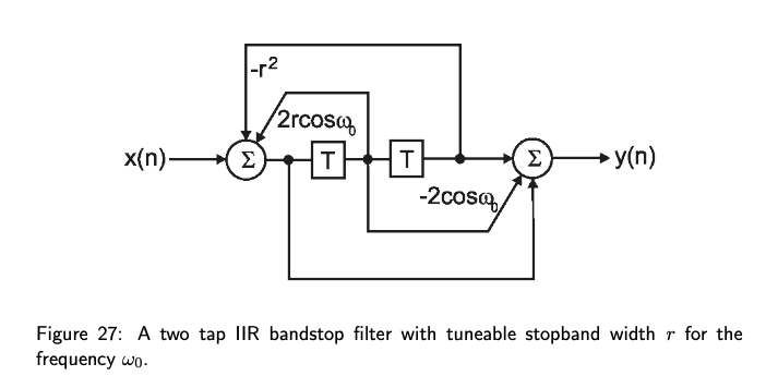
Design of a Pure Digital IIR Notch Filter

$$H(z)=\frac{1-2cos({\omega }_0)z^{-1}+z^{-2}}{1-2r\cos ({\omega }_0)z^{-1}+r^2{z}^{-2}}$$

This gives us a notch filter where the width is tunable while $r<1$ The closer $r$ goes towards 1, the more narrow the frequency reponse.

Link to original

Time or Frequency Response?

Identical frequency response required: Bilinear transform 
Identical temporal behaviour required: Matched z-transform

In most cases the bilinear transform is the transform of choice. The matched z transform can be very useful, for example in robotics where timing is important.

Adaptive IIR, Kalman Filtering

Stability

In summary: poles generate resonances and amplify frequencies. The amplification is strongest the closer the poles move towards the unit circle. The poles need to stay within the unit circle to guarantee stability.

Extra

While zeros knock out frequencies, poles amplify frequencies.

Matched Z-Transform Method

Z-transform \begin{align} z_{\infty}=e^{s_{\infty}T} \\ z_{0}=e^{s_{0}T}\end{align} In the Laplace domain the poles have to be in the left half plane (real value negative). This means that in the sampled domain the poles have to lie within the unit circle. The same rule applies to Zeros

Link to original

Due to this, we know that when $H(s)=s$ turns into $H(z)=1-z^{-1}{e}^{0T}=1-z^{-1}$ which essentially acts like a DC filter

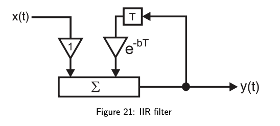
Dataflow Diagram of Simple IIR

Dataflow Diagram of Simple IIR

$h(t)=-e^{-bT}$ So:

$$\begin{array}{rl}Y(z)& =X(z)H(z)\\ & =X(z)\frac{1}{1-e^{-bT}{z}^{-1}}\\ & =Y(z)z^{-1}{e}^{-bT}+X(z)\end{array}$$

We have to recall that $z^{-1}$ is the delay by $T$. With that information we directly have a difference equation in the temporal domain:

$$y(nT)=y([n-1]T)e^{-bT}+x(nT)$$

This means that the output signal $y(nT)$ is calculated by adding the weighted and delayed output signal $y([n-1]T)$ to the input signal $x(nT)$.

Link to original

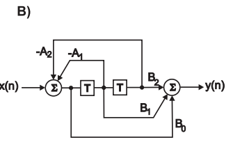
Filter Topologies

In the real world we typically use or chain 2nd order IIR filters:

• There are neat optimisation tools for this
• Higher order filters can be unstable, but making a chain of 2nd order filters is comparatively trivial.
• Complex conjugate pauirs generate naturally in the analogue design, and these directly translate to 2nd order IIR structures.

Simple Direct Form II IIR Filter

class IIR_filter: 
	def __init__(self,_num,_den):
		self.numerator = _num 
		self.denominator = _den 
		self.buffer1 = 0 
		self.buffer2 = 0 
		
	def filter(self,v): 
		input=0.0 
		output=0.0 
		input=v
		output=(self.numerator[1]*self.buffer1) 
		input=input-(self.denominator[1]*self.buffer1) 
		output=output+(self.numerator[2]*self.buffer2) 
		input=input-(self.denominator[2]*self.buffer2) 
		output=output+input*self.numerator[0] 
		self.buffer2=self.buffer1 
		self.buffer1=input 
		return output

In this case our 2 delay steps are just represented by buffer1 and buffer2

In order to achive higher order filters one can then just chain these 2nd order filters. In Python this can be achieved by storing these in an array of instances of this class

Filter Design Based on Analogue Filters

Most IIR filters are designed from analogue filters by transforming from the continuous domain $(h(t),H(s))$ to the sampled domain $(h(n),H(z))$.

Popular Analogue Transfer Functions for IIR Design

Butterworth Filter

All poles lie on the left half plane equally distributed on a half circle with radius $\Omega =2\pi F$ which is shown above. The Butterworth filter is by far the most popular filter. Here are its properties:

• monotonic frequency response
• only poles, no zeros
• the Poles have analytical solution and very easy to calculate
• no constant group delay but usually acceptable deviation from a strict constant group delay for many applications.

Link to original

Chebyshev Filters

Formula:

$$|H(\Omega ){|}^2=\frac{1}{1-{ϵ}^2{T}_n(\Omega /{\Omega }_p)}$$

Where T = Chebyshev polynomials, and these filters have either ripples in the stop or passband depending on the choice of polynomial. As with Butterworth Filters the polynomials have analytical solutions for the poles and zeros of the filter so that their design again is straightforward

Link to original

Bessel Filter

• Constant Group Delay
• Shallow Transition from stop to passband
• No analytical solution for the poles/zeros

Link to original

How to transform the analogue lowpass filters into highpass, bandstop or bandpass filters? All the analogue transfer functions above are lowpass filters. However this is not a limitation because there are handy transforms which take an analogue lowpass transfer function or poles/zeros and then transforms them into highpass, bandpass and stopband filters. These rules can be found in any good analogue filter design book and industry handouts, for example from Analog Devices.

Bilinear Transform

transforming the analogue transfer function into a digital one

As a next step, we need to transform our analogue transfer functions $H(s$) to digital ones $H(z)$

This can be done with the Matched Z-Transform Method, however, the problem is that these map frequencies 1:1 between the analogue and digital domains, which isn’t right due to the Nyquist frequency, which means we cant deal with things such as infinite frequencies. The solution to this is essentially to map all analogue frequencies from $0..\infty$ to $\mathrm{0..0.5}$ in a non-linear way:

$$-\infty <\Omega <\infty ⟹-\pi \le \omega \le \pi$$

This is called the Bilinear Transform:

$$s=\frac{2}{T}\frac{z-1}{z+1}$$

This rule replaces all $s$ with $z$ in our analogue transfer function so that it’s now digital. However, the cutoff frequency ${\Omega }_c$ is still an analogue one but if we want to design a digital filter we want to specify a digital cutoff frequency. Plus remember that the frequency mapping is non-linear so that there is non-linear mapping also of the cutoff.

In the analogue domain the frequency is given as $s=j\Omega$ and in the sampled domain as $z=e^{j\omega }$. Therefore with this we can express:

Core Formula

$$\begin{array}{c}j\Omega =\frac{2}{T}\left[\frac{e^{j\omega }-1}{e^{j\omega }+1}\right]=\frac{2}{T}j\tan \frac{\omega }{2}\\ \Omega =\frac{2}{T}\tan \frac{\omega }{2}\\ \therefore {\Omega }_c=\frac{2}{T}\tan \frac{{\omega }_c}{2}\end{array}$$

Where $T$ is our sampling interval. This also has the benefit of meaning we can express in terms of normalised frequencies using ${\omega }_c=2\pi f_c$

Link to original