Eng Opt Scrapbook

Engineering Optimisation Tutorial 1

Lecture 2

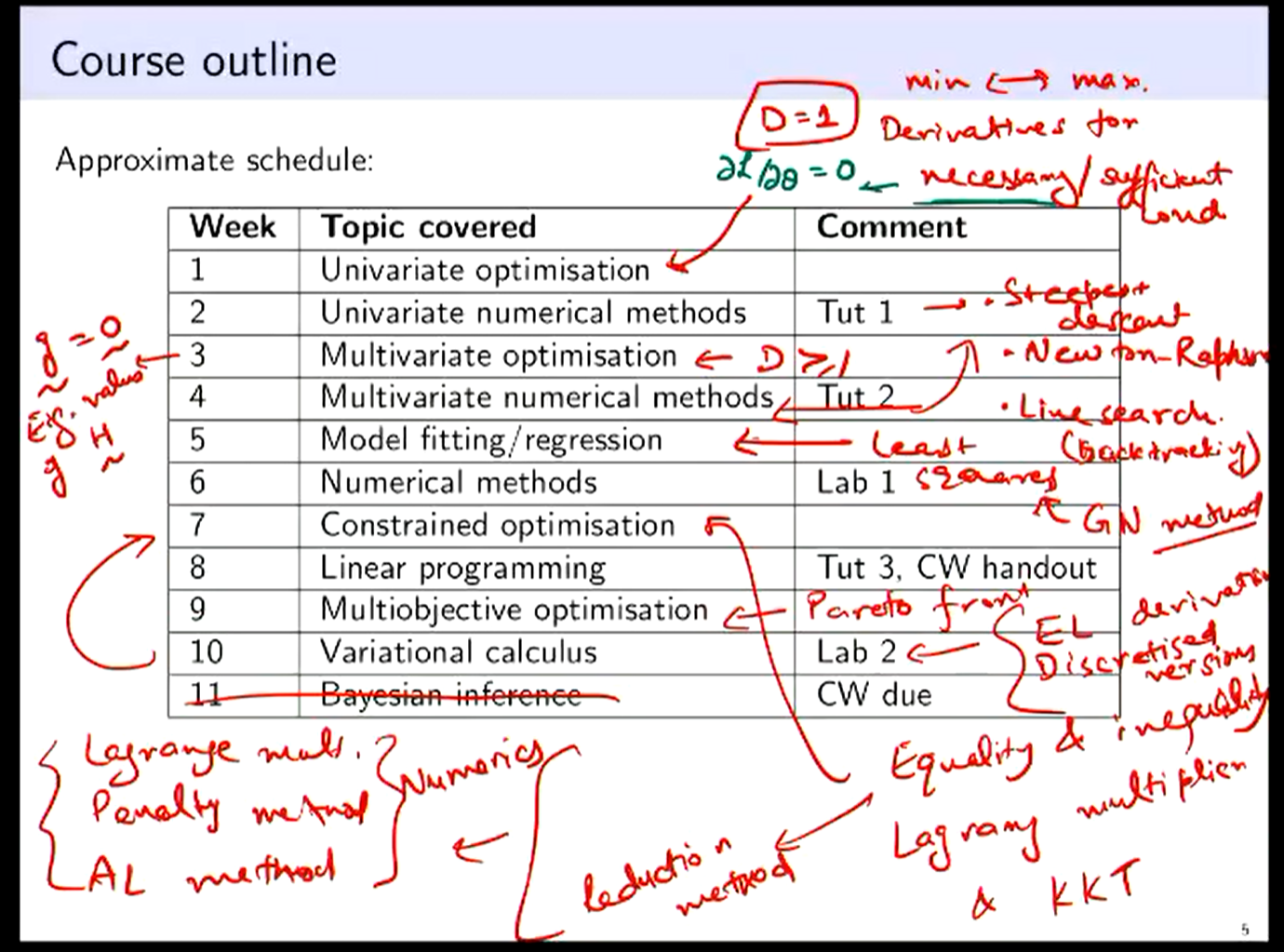
Notes from l1:

• We can approx Hessian with finite diff, such as using secant

For multivariate, $\mathcal{L}(\mathbf{\theta })$ where $\mathbf{\theta }$ is bold, and we are now considering that $\theta \in {\Re }^D$ and that $\mathcal{L}:{\Re }^D\to \Re$

Lecture 3

$$\mathcal{L}(\tilde{\theta })={\theta }_1-{\theta }_2+2{\theta }_1^2+2{\theta }_1{\theta }_2+{\theta }_2^2$$ $$\tilde{g}(\tilde{\theta })=\left[\begin{array}{c}\partial \mathcal{L}/\partial {\theta }_1\\ \partial \mathcal{L}/\partial {\theta }_2\end{array}\right]=\left[\begin{array}{c}1+4{\theta }_1+2{\theta }_2\\ -1+2{\theta }_1+2{\theta }_2\end{array}\right]$$ $$\text{Starting Guess: }\widetilde{{\theta }_o}=\left[\begin{array}{c}0\\ 0\end{array}\right]\Rightarrow g_o=\left[\begin{array}{c}1\\ -1\end{array}\right]$$ $$\Delta \tilde{\theta }=-\alpha \widetilde{g_o}=\left[\begin{array}{c}-\alpha \\ +\alpha \end{array}\right]$$ $${\tilde{\theta }}_1=\left[\begin{array}{c}0-\alpha \\ 0+\alpha \end{array}\right]=\left[\begin{array}{c}-\alpha \\ +\alpha \end{array}\right]$$ $$\hat{\mathcal{L}}(\alpha )=\mathcal{L}(-\alpha ,\alpha )=-\alpha +\alpha +2(-\alpha {)}^2+2(-\alpha )(\alpha )+{\alpha }^2={\alpha }^2$$

Finding $\alpha$ here is called Line Search

Chapter 3 SS Rao Book

Hessian:

$$\mathcal{L}(\tilde{\theta })={\theta }_1-{\theta }_2+2{\theta }_1^2+2{\theta }_1{\theta }_2+{\theta }_2^2$$ $$\tilde{g}(\tilde{\theta })=\left[\begin{array}{c}\partial \mathcal{L}/\partial {\theta }_1\\ \partial \mathcal{L}/\partial {\theta }_2\end{array}\right]=\left[\begin{array}{c}1+4{\theta }_1+2{\theta }_2\\ -1+2{\theta }_1+2{\theta }_2\end{array}\right]$$ $$\tilde{H}(\tilde{\theta })=\left[\begin{array}{cc}\partial {\mathcal{L}}^2/\partial {\theta }_1^2& \partial {\mathcal{L}}^2/\partial {\theta }_1\partial {\theta }_2\\ \partial {\mathcal{L}}^2/\partial {\theta }_2\partial {\theta }_1& \partial \mathcal{L}/\partial {\theta }_2^2\end{array}\right]=\left[\begin{array}{cc}4& 2\\ 2& 2\end{array}\right]$$ $$\text{Starting Guess: }\widetilde{{\theta }_o}=\left[\begin{array}{c}0\\ 0\end{array}\right]\Rightarrow g_o=\left[\begin{array}{c}1\\ -1\end{array}\right]$$ $$\tilde{H}({\theta }_o)\Delta \tilde{\theta }=-{\tilde{g}}_o\Rightarrow \left[\begin{array}{cc}4& 2\\ 2& 2\end{array}\right]\left[\begin{array}{c}\Delta {\theta }_1\\ \Delta {\theta }_2\end{array}\right]=-\left[\begin{array}{c}1\\ -1\end{array}\right]$$

4d1 + 2d2 = -1 2d1 + 2d2 = +1 2d1 = -2 ⇒ d1 = -1 ⇒ d2 = 3/2 $\Delta \tilde{\theta }=\left[\begin{array}{c}\Delta {\theta }_1\\ \Delta {\theta }_1\end{array}\right]=\left[\begin{array}{c}-1\\ 3/2\end{array}\right]$ or

$$\Delta \tilde{\theta }=\left[\begin{array}{c}\Delta {\theta }_1\\ \Delta {\theta }_2\end{array}\right]={\left[\begin{array}{cc}4& 2\\ 2& 2\end{array}\right]}^T\left[\begin{array}{c}-1\\ +1\end{array}\right]=\frac{1}{4}\left[\begin{array}{cc}2& -2\\ -2& 4\end{array}\right]\left[\begin{array}{c}-1\\ +1\end{array}\right]=\frac{1}{4}\left[\begin{array}{c}4\\ 6\end{array}\right]=\left[\begin{array}{c}1\\ 3/2\end{array}\right]$$

Lecture 4

From the problem sheet

$$\underset{\text{matrix}}{\underbrace{\tilde{H}}}={\nabla }_{({\theta }_1,{\theta }_2,{\theta }_3,{\theta }_4)}^2\mathcal{L}=\left[\begin{array}{cccc}\frac{{\partial }^2\mathcal{L}}{\partial {\theta }_1^2}& \frac{{\partial }^2\mathcal{L}}{\partial {\theta }_1\partial {\theta }_2}& \frac{{\partial }^2\mathcal{L}}{\partial {\theta }_1\partial {\theta }_3}& \frac{{\partial }^2\mathcal{L}}{\partial {\theta }_1\partial {\theta }_4}\\ \frac{{\partial }^2\mathcal{L}}{\partial {\theta }_2\partial {\theta }_1}& \frac{{\partial }^2\mathcal{L}}{\partial {\theta }_2^2}& \frac{{\partial }^2\mathcal{L}}{\partial {\theta }_2\partial {\theta }_3}& \frac{{\partial }^2\mathcal{L}}{\partial {\theta }_2\partial {\theta }_4}\\ \frac{{\partial }^2\mathcal{L}}{\partial {\theta }_3\partial {\theta }_1}& \frac{{\partial }^2\mathcal{L}}{\partial {\theta }_3\partial {\theta }_2}& \frac{{\partial }^2\mathcal{L}}{\partial {\theta }_3^2}& \frac{{\partial }^2\mathcal{L}}{\partial {\theta }_3\partial {\theta }_4}\\ \frac{{\partial }^2\mathcal{L}}{\partial {\theta }_4\partial {\theta }_1}& \frac{{\partial }^2\mathcal{L}}{\partial {\theta }_4\partial {\theta }_2}& \frac{{\partial }^2\mathcal{L}}{\partial {\theta }_4\partial {\theta }_3}& \frac{{\partial }^2\mathcal{L}}{\partial {\theta }_4^2}\end{array}\right]$$

Hessian is symmetric so we need $D(D+1)/2$ terms, or $1.5(D^2+D)$ or $30$

Lecture 5

For least squares we need N (num points) to be greater than or equal to D (the dimension) for there to be unique solutions, at N=D we have always a perfect solution (think a line between two points in 2D)

Gauss Newton always descends, even when Newton doesnt, which is interesting, given that it uses only approximation.

A combo of Gauss Newton and steepest descent is called Levenberg - Marquard method

We can define the “error” by least square as residuals and we try to optimise the objective function based on the residual

$$\mathcal{L}(\mathbf{\theta })=\frac{1}{2}\sum _i^N(\mathcal{Y}(x_i;\theta )-y_i{)}^2=\frac{1}{2}\sum r_i^2=\frac{1}{2}||\tilde{r}|{|}^2$$

Called L2 Norm because we are taking square of the components then summing. Other options:

• L1 Norm: $\frac{1}{2}\sum |r_i|$
• L$\infty$ norm: $\frac{1}{2}\max (|r_i|)$

Outlier can significantly distort the “best” result with the L2 norm. Because we’re squaring the residual, meaning that single outliers skew the data much more

l6

if $N<D=>J^{T}J$ is singular ⇒ Solution if not unique, therefore it depends on the initial guess.

Even without a perfect fit in N >> D, it will converge in a single step, its dependent on the gradient not the residual. Doesnt mean its a good fit though…

Rosenbrock function as an example for testing minimization algorithms

L_p norm is denoted as $||\tilde{r}|{|}_p={\sum }_i|r_i{|}^p$ In terms of difficulty: Unconstrained Optimisation < Equality Constraint < Inequality Constraint

l7

Constrained Optimisation | \ __ By Reduction? (If Possible) \ __ Lagrange Multiplier (Take it to a higher dimension) ${\mathcal{L}}^{\ast }=\mathcal{L}-{\sum }_{l=1}^{n_c}{\lambda }_i{c}_i$

Active vs Inactive constraint, for inequalities, if our solution lies on the constraint (active, its basically an equality constraint, but if it doesnt, its an inactive constraint.

KKT condition is an extension of Lagrange, allowing for uncertainty on whether our constraints are active.

$$\begin{array}{c}\mathcal{L}\left({\theta }_1,{\theta }_2\right)={\left({\theta }_1-2\right)}^2+{\left({\theta }_2-1\right)}^2\\ \\ {\theta }_1^2-{\theta }_2⩽0\Rightarrow {\theta }_2-{\theta }_1^2⩾0\\ {\theta }_1+{\theta }_2⩽2\Rightarrow 2-{\theta }_1-{\theta }_2⩾0\\ \\ {\mathcal{L}}^L\left({\theta }_1,{\theta }_2,{\lambda }_1,{\lambda }_2\right)={\left({\theta }_1-2\right)}^2+{\left({\theta }_2-1\right)}^2+{\lambda }_1\left({\theta }_2-{\theta }_1^2\right)+{\lambda }_2\left(2-{\theta }_1-{\theta }_2\right)\\ \\ \\ \text{KKT Conditions: { }\begin{array}{l}\frac{\partial R^L}{\partial {\theta }_1}=0\\ \frac{\partial {\mathcal{L}}^L}{\partial {\theta }_2}=0\end{array}\begin{array}{r}\&{\lambda }_1⩾0\&{\lambda }_2⩾0\\ \left({\theta }_2-{\theta }_1^2\right)⩾0\&\left(2-{\theta }_1-{\theta }_2\right)⩾0\\ {\lambda }_1\left({\theta }_2-{\theta }_1^2\right)=0\&{\lambda }_2\left(2-{\theta }_1-{\theta }_2\right)=0\end{array}\end{array}$$

Augmented Lagrange uses both Lagrange and penalty methods

In unconstrained optimisation: $\mathcal{L}:{\Re }^D\to \Re$ we therefore have D “knobs” to turn. Gradient in any direction should be equal to 0 at minimum ⇒ ${\Delta }_{\theta }\mathcal{L}=\tilde{0}$

Variational calculus Functional Optimisation

l8

Penalty method

$$\begin{array}{rl}& \underset{{\mathcal{L}}_p=x^2+\mu (x-1{)}^2}{\underbrace{\underset{x}{\min }{x}^2\text{ s.t. }x=1}}\\ & \text{True solution: }x=1\\ & \begin{array}{rl}& \underset{x}{\min }{\mathcal{L}}_p\Rightarrow \\ & \text{ Gradient }=\frac{\partial R_p}{\partial x}\\ & =2x+\mu 2(x-1)=0\\ & \Rightarrow x^{\ast }=\frac{\mu }{\mu +1}\end{array}\\ & \text{ if }\mu =1\Rightarrow x^{\ast }=0.5\\ & \mu =10\Rightarrow x^{\ast }=\frac{10}{11}\approx 0.97\end{array}$$

As mu increases, we converge towards 1, but slowly

Penalty Method	Langrange Method
Inexact Solution	Exact Solution
Choosing $\mu$ is non trivial	Saddle Problem
$L_p(x)=x^2+\mu (x-1{)}^2$	$L^L(x,\lambda )=x^2-\lambda (x-1)$

$$L_{AL}=(x;\lambda )=x^2-\lambda (x-1)+\mu (x-1{)}^2$$

Assume $\lambda =0\&\mu =1$ Solve for $x^{\ast }$ $\lambda \leftarrow \lambda -\frac{\mu }{2}(x-1)$ Update $\lambda$

(1) $\lambda =0,\mu =1\Rightarrow x^{\ast }=0.5$

Update $\lambda =0-\frac{1}{2}(0.5-1)=0.25$ (2)

$$\begin{array}{rl}{L}_{AL}(x)=& x^2-0.25(x-1)+1(x-1{)}^2\\ \text{Gradient }=& 2x-0.25+2(x-1)=0\\ & x=\frac{2+0.25}{4}=0.575\end{array}$$

For this:

\mathcal{L}_A(\theta, \lambda, \sigma, \mu) &= L(\theta) - \sum_{j=1}^{m} \lambda_j \epsilon_j(\theta) + \mu \sum_{j=1}^{m} \epsilon_j^2(\theta) \\&\quad- \sum_{k=1}^{n} \lambda_{m+k} I_k(\theta) + \mu \sum_{k=1}^{n} \max(0, -I_k(\theta) )^2 \end{align}

where m is the amount of constrained conditions, and n is the inequality conditions

l9

Wednesday Mar 19th talks about exam

, used for shorthand for derivate:

$${\mathcal{L}}_{,i}\equiv \frac{\partial \mathcal{L}}{\partial {\theta }_i}$$

Backtracking Question Example

$$f(x)=2x_1^2+x_2^2-2x_1{x}_2+x_1-x_2$$

Start at point $x_0=[2,1{]}^{⊺}$, and calculate $\nabla f(x_0)$ and steepest descent direction $p_0$

$$\nabla f(x)=\left\{\begin{array}{c}4x_1-2x_2+1\\ 2x_2-2x_1-1\end{array}\right\}$$ $$\nabla f(x_0)=\left\{\begin{array}{c}8-2+1\\ 2-4-1\end{array}\right\}=\left\{\begin{array}{c}7\\ -3\end{array}\right\}$$ $$p_0=-\nabla f(x_0)=\left\{\begin{array}{c}-7\\ 3\end{array}\right\}$$

(b) Implement one iteration of backtracking line search with parameters ${\alpha }_0=1,\rho =0.5$, and $c=0.3$ to find a suitable step size. Show all iterations of the backtracking procedure. [7 marks]

$$f(x_0+{\alpha }_{0}p)\le f(x_0)+c\alpha \nabla f(x_0{)}^{⊺}{p}_0$$

$f(x_0+{\alpha }_{0}p)=f\left(\left[\begin{array}{c}-5\\ 4\end{array}\right]\right)=50+16+40-5-4=97$ $f(x_0)=8+1-4+2-1=6$ $\alpha c\nabla f(x_0{)}^{⊺}\ast p_0=0.3\ast [7,-3]\ast [-7,3]=0.3\ast -58=-17.4$

Alpha too large! $\alpha =0.5$

For $\alpha =0.5$ :

$$\begin{array}{rl}& x_0+\alpha p_0=[2,1]+0.5\cdot [-7,3]=[-1.5,2.5]\\ & f([-1.5,2.5])=2(-1.5{)}^2+(2.5{)}^2-2(-1.5)(2.5)+(-1.5)-2.5=4.5+6.25+\\ & 7.5-1.5-2.5=14.25\end{array}$$

Check Armijo: $14.25\le 6+0.3\cdot 0.5\cdot (-58)=6-8.7=-2.7$ The condition is still not satisfied. Reduce $\alpha$ again: For $\alpha =0.25$ :

$$\begin{array}{rl}& x_0+\alpha p_0=[2,1]+0.25\cdot [-7,3]=[0.25,1.75]\\ & f([0.25,1.75])=2(0.25{)}^2+(1.75{)}^2-2(0.25)(1.75)+0.25-1.75=0.125+\\ & 3.0625-0.875+0.25-1.75=0.8125\end{array}$$

Check Armijo: $0.8125\le 6+0.3\cdot 0.25\cdot (-58)=6-4.35=1.65$ Since $0.8125\le 1.65$, the Armijo condition is satisfied. We accept $\alpha =0.25$.

Question 2: BFGS Method [20 marks]

Consider the function $f(x)=(x_1-2{)}^2+2(x_2-1{)}^2$ and we are using the BFGS method to minimize it.

(a) Starting with the initial point $x_0=[0,0{]}^T$ and initial Hessian approximation $B_0=I$ (the identity matrix), calculate the first search direction $p_0$ and verify it is a descent direction. [4 marks]

(b) Assuming an exact line search gives a step size of ${\alpha }_0=1$, find the new point $x_1$ and calculate the gradient at this point. [4 marks]

(c) Using the BFGS update formula, compute the new Hessian approximation $B_1$. Show all steps in your calculation. [8 marks]

(d) Calculate the second search direction $p_1$ using the updated Hessian approximation. [4 marks]

Solution 2:

(a) First search direction

For the function $f(x)=(x_1-2{)}^2+2(x_2-1{)}^2$, the gradient is: $\nabla f(x)=\left[\begin{array}{c}2(x_1-2)4(x_2-1)\end{array}\right]$

At $x_0=[0,0{]}^T$: $\nabla f(x_0)=\left[\begin{array}{c}2(0-2)4(0-1)\end{array}\right]=\left[\begin{array}{c}-4-4\end{array}\right]$

With $B_0=I$, the search direction is: $p_0=-B_0^{-1}\nabla f(x_0)=-I^{-1}\left[\begin{array}{c}-4-4\end{array}\right]=\left[\begin{array}{c}44\end{array}\right]$

To verify this is a descent direction, we check that $\nabla f(x_0{)}^T{p}_0<0$: $\nabla f(x_0{)}^T{p}_0=[-4,-4]\cdot [4,4]=-16-16=-32<0$

Therefore, $p_0$ is indeed a descent direction.

(b) New point and gradient

Using step size ${\alpha }_0=1$: $x_1=x_0+{\alpha }_0{p}_0=[0,0]+1\cdot [4,4]=[4,4]$

Calculate the gradient at $x_1$: $\nabla f(x_1)=\left[\begin{array}{c}2(4-2)4(4-1)\end{array}\right]=\left[\begin{array}{c}412\end{array}\right]$

(c) BFGS update

For the BFGS update, we need:

• $s_0=x_1-x_0=[4,4]-[0,0]=[4,4]$
• $y_0=\nabla f(x_1)-\nabla f(x_0)=[4,12]-[-4,-4]=[8,16]$

Now we can use the BFGS update formula: $B_1=B_0-\frac{B_0{s}_0{s}_0^T{B}_0}{s_0^T{B}_0{s}_0}+\frac{y_0{y}_0^T}{y_0^T{s}_0}$

Calculate each term:

• $B_0{s}_0=I\cdot [4,4]=[4,4]$
• $s_0^T{B}_0{s}_0=[4,4]\cdot [4,4]=16+16=32$
• $B_0{s}_0{s}_0^T{B}_0=[4,4]\cdot [4,4{]}^T=\left[\begin{array}{ccc}16& 1616& 16\end{array}\right]$
• $y_0^T{s}_0=[8,16]\cdot [4,4]=32+64=96$
• $y_0{y}_0^T=[8,16]\cdot [8,16{]}^T=\left[\begin{array}{ccc}64& 128128& 256\end{array}\right]$

Substituting: $B_1=I-\frac{1}{32}\left[\begin{array}{ccc}16& 1616& 16\end{array}\right]+\frac{1}{96}\left[\begin{array}{ccc}64& 128128& 256\end{array}\right]$

$B_1=\left[\begin{array}{ccc}1& 00& 1\end{array}\right]-\left[\begin{array}{ccc}0.5& 0.50.5& 0.5\end{array}\right]+\left[\begin{array}{ccc}0.667& 1.3331.333& 2.667\end{array}\right]$

$B_1=\left[\begin{array}{ccc}1.167& 0.8330.833& 3.167\end{array}\right]$

(d) Second search direction

To find the second search direction, we need to solve the system $B_1{p}_1=-\nabla f(x_1)$:

$\left[\begin{array}{ccc}1.167& 0.8330.833& 3.167\end{array}\right]p_1=-\left[\begin{array}{c}412\end{array}\right]$

We can find $p_1$ by computing $B_1^{-1}$: $\det (B_1)=1.167\cdot 3.167-0.833\cdot 0.833=3.027$

$B_1^{-1}=\frac{1}{3.027}\left[\begin{array}{ccc}3.167& -0.833-0.833& 1.167\end{array}\right]=\left[\begin{array}{ccc}1.046& -0.275-0.275& 0.386\end{array}\right]$

Therefore: $p_1=-B_1^{-1}\nabla f(x_1)=-\left[\begin{array}{ccc}1.046& -0.275-0.275& 0.386\end{array}\right]\left[\begin{array}{c}412\end{array}\right]$

$p_1=-\left[\begin{array}{c}4.184-3.3-1.1+4.632\end{array}\right]=-\left[\begin{array}{c}0.8843.532\end{array}\right]=\left[\begin{array}{c}-0.884-3.532\end{array}\right]$

This is the second search direction according to the BFGS method.