Pros:
TCP Reno is effective at keeping bottleneck link fully utilised
- Trades some extra delay to maintain throughput
- Provided sufficient buffering in the network: buffer size = bandwidth × delay
- Packets queued in buffer → delay
Cons:
- Assumes packet loss is due to congestion; non-congestive loss, e.g., due to wireless interference, impacts throughput
- Congestion avoidance phase takes a long time to use increased capacity
Sliding Window Protocols
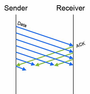
Sliding window protocols improve link utilization using a congestion window – number of packets to be sent before an acknowledgement arrives.
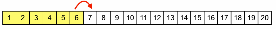
 In this example, the window size is six packets → acknowledgement for packet 6 arrives just in time to release packet 7 for transmission
Each returning acknowledgement for new data slides the window along, releasing next packet for transmission → if window sized correctly, each acknowledgement arrives just in time to release next packet This means that ideally just as/ just after the last packet comes in, the acknowledgement for the first packet comes in.
What is the optimal size for the window? bandwidth × delay of path → but neither is known to the sender
The delay will be changed by the slowest link, but we don’t know our path. So we have to guess:
How to choose initial window size, ?
- No information → need to measure path capacity
- Start with a small window, increase until congestion
- = 1 packet per round-trip time (RTT) is safe
- Start at the slowest possible rate, equivalent to stop-and-wait, and increase
- = 3 packets per RTT - **Traditional TCP Reno approach **
- = 10 packets per RTT - Modern TCP implementations [RFC 6928]
- Compromise between safety and performance – measurements show this is generally safe at present
- Expect to gradually be increased as average network performance improves
Two Stage Send Model:
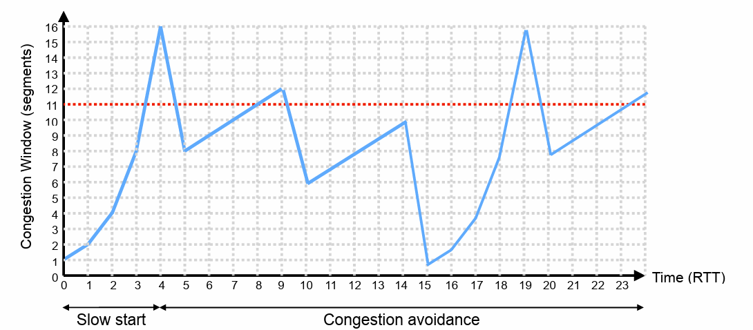
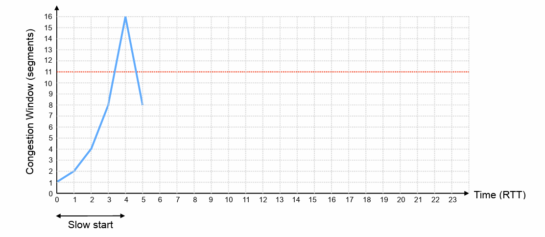
Slow Start
Deceptively named:
- Assume = 1 packet per RTT – slow start to connection
- It will be = 3 or = 10 in practice, but using = 1 makes the example simpler…
- Rapidly increase window until network capacity is reached
- Each acknowledgement for new data increases congestion window, W, by 1 packet per RTT → congestion window doubles each RTT
- If a packet is lost, halve congestion window back to previous value and exit slow start
Congestion Avoidance
After first packet is lost, TCP switches to congestion avoidance
- The congestion window is now approximately the right size for the path
- Goal is now to adapt to changes in network capacity
- Perhaps the path capacity changes – radio signal strength changes for mobile device
- Perhaps the other traffic changes – competing flows stop; additional cross-traffic starts
- Additive increase, multiplicative decrease of congestion window
If a complete window of packets is sent without loss:
- Increase congestion window by 1 packet per RTT, then send next window worth of packets
- Slow, linear, additive increase in window:
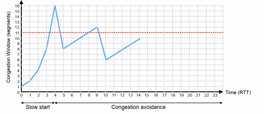 If a packet is lost and detected via triple duplicate acknowledgement:
- Transient congestion, but data still being received
- Multiplicative decrease in window:
- Rapid reduction in window allows congestion to clear quickly, avoids congestion collapse
- Then, return to additive increase until next loss
If a packet is lost and detected via timeout:
• Either receiver or path has failed – reset to and re-enter slow start
• How long is the timeout?
• =
If a packet is lost and detected via triple duplicate acknowledgement:
- Transient congestion, but data still being received
- Multiplicative decrease in window:
- Rapid reduction in window allows congestion to clear quickly, avoids congestion collapse
- Then, return to additive increase until next loss
If a packet is lost and detected via timeout:
• Either receiver or path has failed – reset to and re-enter slow start
• How long is the timeout?
• =