Jump To
Past Papers
Transclude of Control32016PP.excalidrawControl 3 2023 Past Paper
Sept 1999
Q5:
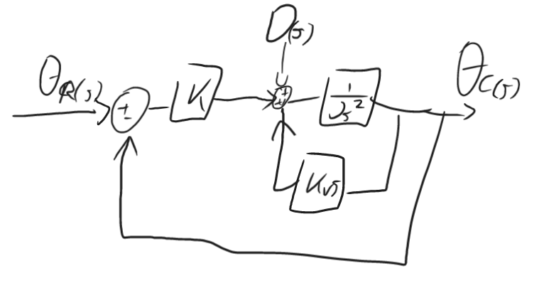
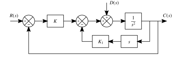
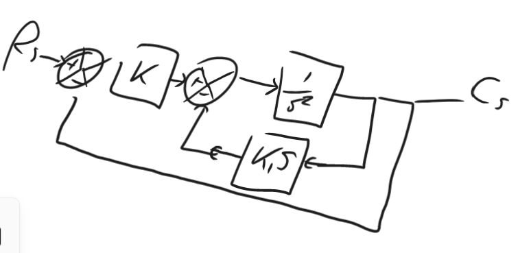
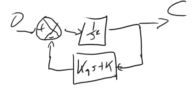
The block diagram drawn is of a satellite attitude control system. The reference attitude is , while the actual attitude is denoted by . The satellite has a moment of Inertia, , about its axis of rotation, whilst and are control system gains. The control system also acts to eliminate unwanted rotations due to a disturbance torque .
a) Derive the transfer function relating actual attitude to reference, b) Derive the transfer function relating actual attitude to disturbance, c) A ref input consisting of a step change of is applied at the same instant the satellite experiences a disturbance equiv to a step change of Nm. Given the following values, derive an expression for the satellite’s attitude due to the following inputs:
Solution
a) Taking to be 0, we get a feedback of over , meaning this can be simplified to: , this subsequently cascades with giving us , which finally has a unity gain, meaning that:
b) Taking to be 0, we get a feedback of over , which means that:
c) If we take
\begin{align} \theta_c(s) &= \frac{500*(\frac{5\pi}{180})+\frac{50}{s}}{s(25s^2+100s+500)} = \frac{\frac{100\pi}{180s} + \frac{2}{s}}{s(s^2+4s+20)}\\ &= \frac{A}{s} + \frac{Bs+C}{s^2+4s+20} \\\\ 1 &= A(s^2+4s+20) + s(Bs+C) \\ 1&=(A+B)s^2 + (4A+C)s + (20)A \\ s^0 &: 1 =20A, A=1/20 \\ s^1 &: 0 =(4A+C), C=-4/20 \\ s^2 &: 0 = (A+B) , B=-1/20 \\ \therefore\theta_c(s) &= \frac{3.7454}{20}[\frac{1}{s} - \frac{s+4}{s^2+4s+20}] \\ & \text{Recognising } s^2+4s+20 = (s+2)^2+4^2 \\ \theta_c(s) &= 0.18727[\frac{1}{s} - \frac{s+2}{(s+2)^2+4^2} - \frac{1}{2}*\frac{4}{(s+2)^2+4^2}] \\ \rightarrow \theta(t)&= 0.18727[1-e^{-2t}(\cos(4t)+\frac{\sin(4t)}{2})] \end{align}
June 1998
Question
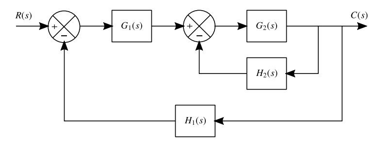
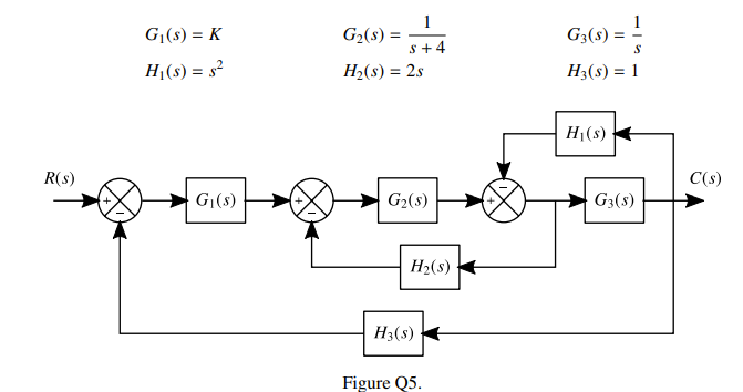
Figure Q.5 shows the block diagram of a control system.
a) Using block diagram reduction techniques determine the closed loop transfer function of the system shown in Figure Q5.
b) Given the individual transfer functions listed below, using Routh’s criteria determine the range of values of K which for the system to remain stable.
Solution
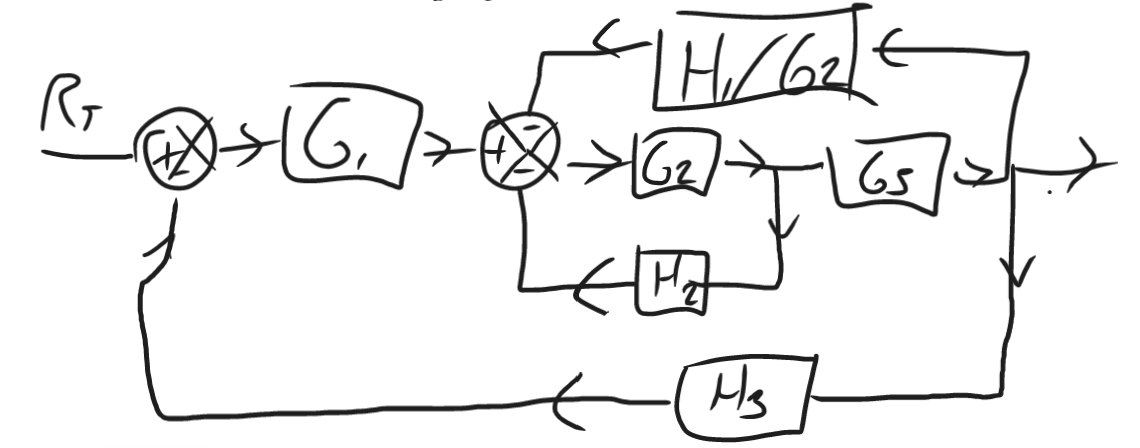
a)
First we can reorganise the block diagram, moving the summing block in front of behind it:
 Now we can tackle this standardly:
this then cascades with :
This block now has in feedback with it:
This now cascades with :
This block now has in feedback, giving:
Now we can tackle this standardly:
this then cascades with :
This block now has in feedback with it:
This now cascades with :
This block now has in feedback, giving:
b) , \begin{align} \begin{array}{c|ccccc} s^3 & 1 & 4 \\ s^{2} & 7 & K \\ s^{1} & 4-\frac{K}{7} & 0 \\ s^{0} & K \\ \end{array} \end{align}
Tutorials
Block Diagram
Tut 1 Q1:
Question
Figure Q1 shows a block diagram of the positioning control system of the Hubble space telescope. Given that and , derive the closed loop transfer functions relating angular position to both the commanded input and a general disturbance . Determine the response of the telescope to a unit step input in . Hence deduce the telescope’s response to a unit step disturbance .
Solution
First, for calculating , we will take , meaning:
We can eliminate the feedback loop relatively simply:
Then this is in series with giving us:
Finally this is in a unity feedback loop giving us:
For finding we can assume to be 0, and recenter our block diagram around our input:
This is a simple feedback loop: Giving us
For a unit step input in , we get , therefore:
\begin{align} \frac{a}{s} &+ \frac{bs+c}{s^2+12s+100} \\100&= a(s^2+12s+100) + s(bs+c) \\ 100 &= (a+b)s^2 + (12a+c)s + 100a \\ s^0&: 100 = 100a, \quad a =1 \\ s^1 &: 0 = (12+c), \quad c = -12 \\ s^2 &: 0=a+b, \quad b=-1 \\ \therefore C(s)_R &=\frac{100}{s} - \frac{s+12}{s^2+12s+100} \\ &\text{Note that }s^2+12s+100 = (s+6)^2+8^2: \\ C(s)_R &= \frac{100}{s}-\frac{s+6}{(s+6)^2+8} - \frac{6}{8}*\frac{8}{(s+6)^2+8} \\ \therefore c(t)_R &= 100 - e^{-6t}\cos8t - \frac{3e^{-6t}\sin8t}{4} \\ c(t)_R &= 100 - e^{-6t}[\cos8t+\frac{3\sin8t}{4}] \end{align}
Tut 1 Q2:
Question
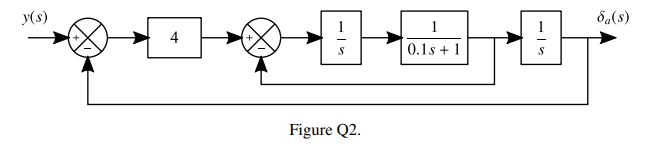
The ailerons of a large airliner are positioned through an angle by servo actuators which respond to the pilot’s lateral stick displacement , Figure Q2. Derive the closed loop transfer function of this system relating the aileron displacement to the pilot’s stick motions.
Solution
We can eliminate the unity feedback over giving us: , which then feeds into another , as well as a term giving us , finally this has a unity feedback meaning the final is:
Tut 1 Q3:
Question
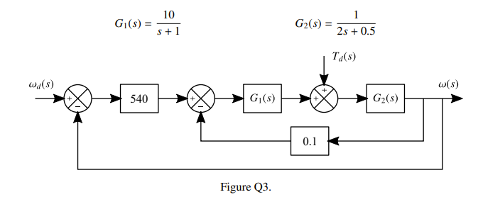
Figure Q3 shows the block diagram of an electric locomotive motor where ωd is the desired angular velocity of motor as set by the driver whilst ω is the actual angular velocity achieved. The block represents the load transfer function (i.e. the locomotive) whilst is the armature controller transfer function. The locomotive motor can experience torque disturbances due to braking, given by . Derive the transfer functions relating output angular velocity to desired angular velocity, and output angular velocity to torque disturbance, , given:
Solution
First to find , we can set , meaning that we have in feedback with 0.1, this becomes , which would now be in series with , this becomes , which finally has unity feedback giving us:
Finding , we set to 0:
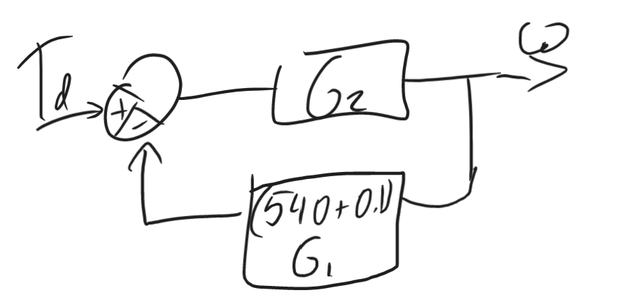 So our is just a feedback loop of with
\begin{align}
\frac{\omega(s)}{T_d(s)} &= \frac{\frac{1}{2s+0.5}}{1+\frac{5401}{(s+1)(2s+0.5)}} = \frac{1}{2s+0.5+\frac{5401}{s+1}} \\&= \frac{s+1}{(2s^2+2s)+(0.5s+0.5)+5401} \\
&=\frac{s+1}{2s^2+2.5s+5401.5} \\
&= \frac{0.5(s+1)}{s^2+1.25s+2,700.75}
\end{align}
So our is just a feedback loop of with
\begin{align}
\frac{\omega(s)}{T_d(s)} &= \frac{\frac{1}{2s+0.5}}{1+\frac{5401}{(s+1)(2s+0.5)}} = \frac{1}{2s+0.5+\frac{5401}{s+1}} \\&= \frac{s+1}{(2s^2+2s)+(0.5s+0.5)+5401} \\
&=\frac{s+1}{2s^2+2.5s+5401.5} \\
&= \frac{0.5(s+1)}{s^2+1.25s+2,700.75}
\end{align}
Tut 1, Q8, Pt1
Question
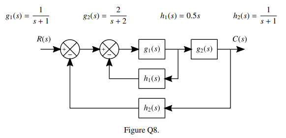
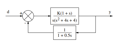
Determine the closed loop transfer function of the system shown in Figure Q8. Investigate the stability of this system when:
Solution
Feedback Loop = , this then cascades with , making , This collective then has a feedback of which makes the full thing: \begin{align} \frac{C(s)}{R(s)} &= \frac{\frac{s}{1.5s^2+4s+2}}{1+\frac{s}{(s+1)(1.5s^2+4s+2)}} = \frac{s}{1.5s^2+4s+2+\frac{s}{s+1}} \\ &= \frac{s(s+1)}{(1.5s^3+4s^2+2s) + (1.5s^2+4s+2) + s} \\ &= \frac{s(s+1)}{1.5s^3+5.5s^2+7s+2} \\ &= \frac{\frac{2}{3}s(s+1)}{s^3 + (11/3 )s^2 +(14/3)s+(4/3)} \end{align}
TF & Stability
Tut 1 Q4:
Question
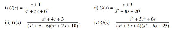
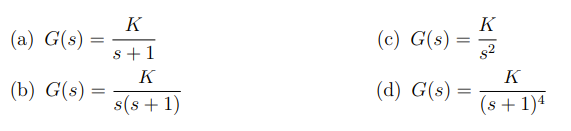
Calculate the poles and zeros of the systems with the following transfer functions. Comment on the stability of each and the expected response characteristics.
Solution
i) Zeros at , Poles at , stable, no oscillations ii) Zeros at , Poles at Stable System, Oscillatory iii) Zeros at , Poles at: . Unstable System, Oscillatory iv) Zeros at …, Poles at: , Unstable System, Oscillatory.
Tut 1 Q5:
Question
Figure Q5 shows a block diagram for a feedback control system. Determine the values of the closed loop poles and hence the stability of the system with the following combinations of controller and plant transfer functions.
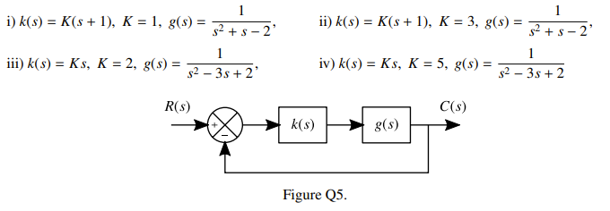
Solution
i) Poles at . Stable System with oscillations.
ii) Poles at . Stable system with oscillations
iii) Poles at , Unstable System, Oscillatory
iv) Poles at . Stable System. Oscillatory
Tut 2, Q1:
Question
A controller with proportional gain is in series with a plant with transfer function and employs a unity negative feedback loop.
a) Determine the response of the system to a unit step input if the feedback loop is open.
b) If the feedback loop is closed, determine the response to a unit step input given: i) = 0.5, ii) = 10.
c) What is the lowest value of which gives a non-oscillatory response?
Solution
a) cascades giving us: Assuming no feedback (open loop), our response to a unit step would be:
\begin{align} \frac{1}{s^2(s+20)} &= \frac{A}{s^2}+ \frac{B}{s} + \frac{C}{s+20} \\ 1 &= A(s+20) + B(s^2+20s) + Cs^2 \\ &= (B+C)s^2 + (A+20B)s + 20A \\ s^0 &: 1 = 20A,\quad A=\frac{1}{20} \\ s^1 &: 0=(A+20B), \quad B =-\frac{1}{400} \\ s^2 &: 0=(B+C), \quad C=\frac{1}{400} \\ \therefore C(s) &= \frac{1}{s^2(s+20)} \\&= 20K_p[\frac{0.05}{s^2} - \frac{0.0025}{s} + \frac{0.0025}{s+20}] \\ \therefore c(t) &= \frac{K_p}{20}[20t-1+e^{-20t}] \end{align}
b) If the feedback loop is closed, with a unity feedback, we get: With a unit step response: i) Solving for factors: \begin{align} C(s)&=\frac{1}{s(s+0.51)(s+19.49)}\\ &= \frac{A}{s}+\frac{B}{s+0.51}+\frac{C}{s+19.49} \\ \text{So:}\\ 1 &=A(s+0.51)(s+19.49) + Bs(s+19.49) + Cs(s+0.51) \\ &= A(s^2+20s+9.94) + B(s^2+19.49s) + C(s^2+0.51s) \\ &= s^2(A+B+C) +s(20A+19.49B+0.51C) + 9.94A \\ \text{Given} & \text{ this:} \\ s^0 &: 1= 9.94A,\quad A = 0.101 \\ s^1 &: 0= 20A+19.49B+0.51C,\quad 19.49B+0.51C = -2.02 \\ s^2 &: 0 = A+B+C, \quad B+C=-0.101 \\ \therefore &\quad 18.98B = -2.02 - (-0.05151) = -1.96849 \\ &\quad B= -0.1037, \quad C=-0.0027 \\ C(s) &= \frac{0.101}{s} -\frac{0.1037}{s+0.51} -\frac{0.0027}{s+19.49} \\ \therefore c(t) &=0.101-0.1037e^{-0.51t}-0.0027e^{-19.49t} \end{align}
c)
System is oscillatory for : Oscillatory for Oscillatory for
Routh’s Criterion
Tut 1, Q6
Question
Use Routh’s Criterion to determine the stability characteristics of the following systems. In each case determine the number of positive roots.

Solution
i) The system is stable
ii) The system is stable
iii) Two sign changes, Two positive roots, unstable system
iv) Two sign changes, Two Positive Roots, unstable system
Tut 1, Q7
Question
Use Routh’s Criterion to determine the range of values of K which give stability for the systems with closed loop characteristic equations:

Solution
i)
ii)
Tut 1, Q8, Pt2
Question
Determine the closed loop transfer function of the system shown in Figure Q8. Investigate the stability of this system when:
Solution
From Part 1 No sign changes indicates that this is a stable system.
Root Locus
Tut 3, Q2:
Using the standard rules, draw the approximate root-locus diagrams for the systems in question Q1.
Tut 3, Q6:
Worked Examples
Block Diagrams
Ex 1: