Point of Instability Analysis

As explained in section 3.7, stability of the closed loop system is a key performance target. We now have a number of tools which allow us to determine the point of instability for a system with a simple varying gain factor

Consider an open-loop system of the form:

$$G(s)=K{G}_o(s)$$

as let us assume that $G_o(s)$ is such that for some value of $K$, the corresponding closed-loop system ($G_c(s)=\frac{G(s)}{1+G(s)}$) becomes unstable.

We have three methods for finding the value of K for which the system becomes unstable, and to determine the corresponding crossing point of the root locus into the right half plane (i.e., the point at which the system becomes unstable).

These are:

1. Using Routh-Hurwitz to determine the value of gain, $K$ , for which the system becomes unstable, and then the magnitude condition to determine the position
2. Use the Angle Criterion of the Root Locus (section 2.1.1) directly and determine the crossing point of the root-locus into the right half-plane. The Calibration Equation (section 2.1.1) can then be used to determine the value of the gain, K, which corresponds to the crossing points, i.e. for which the system becomes unstable.
3. By substituting s = jω in the transfer function and then using the Nyquist Stability Criterion (section 3.6) to determine the gain margin of $G_o(s)$, which is equivalent to the value of K to reach instability.

Example:

We can apply all three of the following to:

$$G(s)=\frac{K}{s(s+1)(s+2)}$$

Routh-Hurwitz The characteristic equation of $G(s)$ can be described as:

$$F(s)=s^3+3s^2+2s+K=0$$

and Routh-Hurwitz gives us two conditions:

• $K>0$ (all coefficients $>0$ )
• $K<6$ ($a_o{a}_3<a_1{a}_2$).

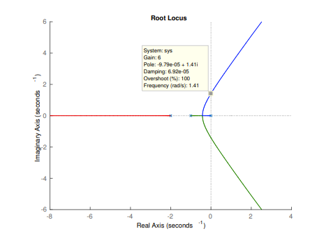
We therefore have the value of $K=6$ as the point of instability. We know that this point is a certain distance up the imaginary axis; let this distance be x, then the magnitude condition gives:

$$K=\frac{{\prod }_1^n\text{ distance to open loop poles }}{{\prod }_1^m\text{ distance to open loop zeros }}=x\times \sqrt{x^2+1}\times \sqrt{x^2+4}=6$$

This can be re-arranged (by squaring both sides of the equation) to:

$$x^2(x^2+1)(x^2+4)-36=x^6+5x^4+4x^2-36=0$$

and a solution of this equation can be found.

There is only one imaginary solution to this equation, which is $x^2=-4$ and hence $x=\pm \sqrt{2}j$The crossing point on the imaginary axis is therefore at $\pm \sqrt{2}j$

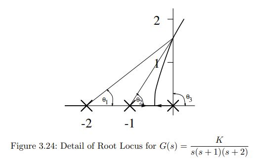
Angle Criterion of Root Locus The angle criterion states that for points on the locus: $\Sigma$ angles subtended from zeros − $\Sigma$ angles subtended from poles = $-180^o\pm k.360^o$

In this case, this results to: $-{\theta }_1-{\theta }_2-{\theta }_3=-{\tan }^{-1}x-{\tan }^{-1}\frac{x}{2}-90^o=-180^o$ Which simplifies to: ${\tan }^{-1}x+{\tan }^{-1}\frac{x}{2}=90^o$

Using the following formula: ${\tan }^{-1}A+{\tan }^{-1}B={\tan }^{-1}\{\frac{A+B}{1-AB}\}$

We can simplify our previous equation to: ${\tan }^{-1}\{\frac{3x/2}{1-x^2/2}\}=90^o$

Therefore: $1-x^2/2=0\Rightarrow x=\pm \sqrt{2}$

As we can see here, we also find the “crossing point” of the $\mathfrak{Im}$ axis.

We can evaluate the value of $K$ that this happens using the magnitude condition:

$$K=\frac{{\prod }_1^n\text{distance to open loop poles}}{{\prod }_1^n\text{distance to open loop zeros}}=\sqrt{2}\ast \sqrt{2+1}\ast \sqrt{2+4}=6$$

Nyquist Frequency Response Plot

Two techniques can be used to determine the crossing point of the negative real axis, which both give the same solution:

1. Find the frequency at which $\mathfrak{Im}\{G(j\omega )\}=0.2$.
2. Find the frequency at which the phase is $-180^o$ , i.e. $\arg (G(j\omega ))=-180^o$

After the frequency is determined the magnitude at that frequency is found from the magnitude equation. Substituting $s=j\omega$ in the transfer function results in:

$$G(j\omega )=\frac{K}{j\omega (j\omega +1)(j\omega +2)}=\frac{K/2}{j\omega (1+j\omega )(1+(j\omega )/2)}$$

This means we can write the magnitude of the freq response as:

$$|G(j\omega )|=\frac{K/2}{\omega \sqrt{1+{\omega }^2}\sqrt{1+{\omega }^2/4}}$$

and the phase as:

$$\arg G(j\omega )=-90^o-ta{n}^{-1}\omega -ta{n}^{-1}\omega /2=-90^o-ta{n}^{-1}\frac{3\omega /2}{1-{\omega }^2/2}$$

1. Using $\mathfrak{Im}\{G(j\omega )\}=0$ gives: \mathfrak{Im}\{G(j\omega)\} &= \mathfrak{Im}\{\frac{K/2}{j\omega(j\omega+1)(j\omega+2)}\} \\ \text{Multiply by} & \text{ complex conjugate:} \\ &= \mathfrak{Im}\{\frac{K/2(-j\omega)(1-j\omega)(1-(j\omega)/2)}{\omega^2(1+\omega^2)(1+\omega^2/4)}\} \\ &= \mathfrak{Im}\{\frac{K/2(-j\omega)(1-(3j\omega)/2-\omega^2/2)}{\omega^2(1+\omega^2)(1+\omega^2/4)}\} \\ &= \frac{K/2(-j\omega +j\omega^3/2)}{\omega^2(1+\omega^2)(1+\omega^2/4)} \\ \text{Equating to} & \text{ zero implies:} \\ & -\omega + \omega^3/2=0 \Rightarrow \omega = 0 \text{ or }\omega=\sqrt2 \end{align} $$
2. Using $\arg G(j\omega )=-180^o$ gives us: ${\tan }^{-1}\frac{\omega /2}{1-{\omega }^2/2}=-90^o$ which implies that: $\frac{\omega /2}{1-{\omega }^2/2}=\infty$ Which therefore means either that: $1-{\omega }^2/2=0,\Rightarrow \omega =\pm \sqrt{2}$ Denoting where our crossing points are

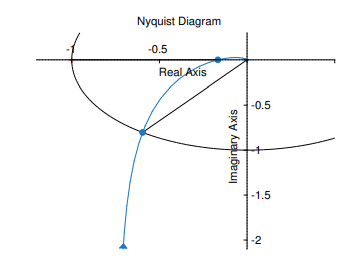
The Nyquist Plot is:

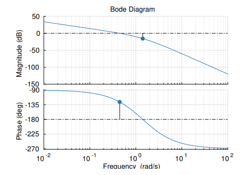
The Bode Plot is: