Cloud computing represents a paradigm shift in how computing resources are delivered, managed, and consumed. It provides on-demand access to a shared pool of configurable computing resources that can be rapidly provisioned and released with minimal management effort.
“A model for enabling ubiquitous, convenient, on-demand network access to a shared pool of configurable computing resources (e.g., networks, servers, storage, applications, and services) that can be rapidly provisioned and released with minimal management effort or service provider interaction.”
Evolution of Distributed Computing
The evolution of distributed computing can be traced through several major paradigms:
Virtualization is the core technology that enables cloud computing by abstracting physical resources into logical units that can be provisioned on-demand. It allows:
Sharing of physical resources among multiple users
Isolation between different workloads
Rapid provisioning and deprovisioning of resources
Cloud providers maintain large pools of resources that are dynamically allocated to customers, creating economies of scale and high utilization rates.
Automation and Self-service
Cloud systems provide automated interfaces (APIs and web portals) that allow users to provision and manage resources without human intervention from the provider.
Elasticity and Scalability
Cloud resources can scale up or down based on demand, creating the illusion of infinite resources while optimizing resource usage.
Challenges for Cloud Providers
Cloud providers face several key challenges:
Rapid provisioning of resources without human interaction
Creating the illusion of infinite resources while managing data centers efficiently
The National Institute of Standards and Technology (NIST) has provided the most widely accepted definition of cloud computing, which has become the standard reference in both industry and academia.
Definition
According to NIST Special Publication 800-145:
“Cloud computing is a model for enabling ubiquitous, convenient, on-demand network access to a shared pool of configurable computing resources (e.g., networks, servers, storage, applications, and services) that can be rapidly provisioned and released with minimal management effort or service provider interaction.”
The Three Dimensions of Cloud Computing
NIST defines cloud computing along three major dimensions:
Five Essential Characteristics
Three Service Models
Four Deployment Models
Five Essential Characteristics
On-demand self-service: Computing capabilities can be provisioned automatically without requiring human interaction with service providers.
Broad network access: Capabilities are available over the network and accessed through standard mechanisms that promote use by heterogeneous client platforms.
Resource pooling: The provider’s computing resources are pooled to serve multiple consumers using a multi-tenant model, with different physical and virtual resources dynamically assigned and reassigned according to consumer demand.
Rapid elasticity: Capabilities can be elastically provisioned and released, in some cases automatically, to scale rapidly outward and inward commensurate with demand.
Measured service: Cloud systems automatically control and optimize resource use by leveraging a metering capability at some level of abstraction appropriate to the type of service.
Three Service Models
Software as a Service (SaaS): The consumer uses the provider’s applications running on a cloud infrastructure. Applications are accessible from various client devices through either a thin client interface or a program interface.
Platform as a Service (PaaS): The consumer deploys consumer-created or acquired applications onto the cloud infrastructure using programming languages, libraries, services, and tools supported by the provider.
Infrastructure as a Service (IaaS): The provider provisions processing, storage, networks, and other fundamental computing resources where the consumer can deploy and run arbitrary software, including operating systems and applications.
Four Deployment Models
Private Cloud: The cloud infrastructure is provisioned for exclusive use by a single organization comprising multiple consumers.
Community Cloud: The cloud infrastructure is provisioned for exclusive use by a specific community of consumers from organizations that have shared concerns.
Public Cloud: The cloud infrastructure is provisioned for open use by the general public.
Hybrid Cloud: The cloud infrastructure is a composition of two or more distinct cloud infrastructures (private, community, or public) that remain unique entities but are bound together by standardized or proprietary technology.
The evolution of distributed computing systems has progressed through various paradigms, each building on the previous while addressing different needs and use cases.
Clusters
A cluster is a group of computers that work together as a unified computing resource.
Key Characteristics:
Homogeneity: Clusters typically consist of similar or identical hardware and software systems
Network: Connected via high-speed, low-latency local area networks
Management: Centrally managed as a single system
Purpose: Improve availability, resource utilization, and price/performance ratio
Examples:
HPC (High-Performance Computing) clusters used in scientific research
Analytics clusters at large tech companies (Google, Microsoft, Meta, Alibaba, Amazon)
Load-balanced web server clusters
Database clusters for high availability
Use Cases:
Compute-intensive scientific simulations
Big data analytics
High-availability services
Grids
Grid computing connects distributed, heterogeneous computing resources across organizational boundaries to solve larger problems.
Key Characteristics:
Heterogeneity: Diverse hardware and software resources across different administrative domains
Distribution: Resources are geographically distributed and connected via wide-area networks (internet)
Standardization: Middleware provides standardized interfaces to access diverse resources
Sharing: Resources are shared across organizations for common goals
Berkeley Open Infrastructure for Network Computing (BOINC)
Earth System Grid Federation (ESGF)
Use Cases:
Large-scale scientific research
Distributed data analysis
Volunteer computing projects
Clouds
Cloud computing provides on-demand access to shared pools of configurable computing resources delivered as a service over a network.
Key Characteristics:
On-Demand Self-Service: Users can provision resources without human interaction from providers
Utility Model: Pay-as-you-go pricing, similar to electricity or water utilities
Resource Pooling: Multi-tenancy with dynamic resource allocation
Elasticity: Ability to scale resources up or down rapidly
Measured Service: Resource usage is monitored, controlled, and reported
Examples:
Amazon Web Services (AWS)
Microsoft Azure
Google Cloud Platform
IBM Cloud
Oracle Cloud
Use Cases:
Web applications and services
Enterprise IT infrastructure
Development and testing environments
Data storage and backup
High-availability and disaster recovery
Comparison
Feature
Clusters
Grids
Clouds
Ownership
Single organization
Multiple organizations
Service providers or organizations
Hardware
Homogeneous
Heterogeneous
Heterogeneous (abstracted)
Location
Co-located
Geographically distributed
Data centers (abstracted from users)
Management
Centralized
Distributed
Centralized for each provider
Scalability
Limited by physical resources
Limited by participating resources
Highly elastic (appears unlimited)
Access
Local network, specific interfaces
Grid middleware, certificates
Standard web protocols, APIs
Business Model
Capital expenditure
Collaborative
Operational expenditure (utility)
Virtualization
Limited
Limited
Extensive
Evolution and Relationship
These paradigms represent an evolution in distributed computing, with each building on concepts from previous approaches:
Clusters provided the foundation for resource pooling and unified management
Grids extended this to distributed resources across organizations
Clouds added virtualization, elasticity, and the utility model
While clouds have become dominant for many use cases, clusters and grids continue to serve specific purposes, especially in scientific and research computing.
Virtualization is the foundation that enables cloud computing by abstracting physical resources into logical units that can be provisioned on-demand.
Definition
According to NIST Special Publication 800-125:
“Virtualization is the simulation of the software and/or hardware upon which other software runs. This simulated environment is called a virtual machine (VM).”
In other words, virtualization creates an abstraction layer that transforms a real (physical) system so it appears as a different virtual system or as multiple virtual systems.
Key Concepts
Host System: The physical hardware and software on which virtualization is implemented
Guest System: The virtual system that runs on the host
Hypervisor/VMM (Virtual Machine Monitor): Software that creates and manages virtual machines
Formal Definition
Virtualization can be formally defined through an isomorphism V that maps the guest state to the host state:
For each sequence of operations e that modifies the guest’s state from Si to Sj
There exists a corresponding sequence of operations e’ that performs an equivalent modification between the host’s states (S’i to S’j)
Categories of Virtualization
Virtualization technologies can be categorized into three main types:
1. Process Virtualization
Creates a virtual environment for individual applications
Examples: Java Virtual Machine (JVM), Common Language Runtime (.NET/Mono)
Used for platform independence and sandboxing
2. OS-Level Virtualization
Creates isolated environments (containers) within an operating system
A Virtual Machine (VM) is a software-based emulation of a physical computer that can run an operating system and applications as if they were running on physical hardware.
Definition
A virtual machine provides an environment that is logically separated from the underlying physical hardware. The hardware elements (CPU, memory, storage, network) presented to the VM are abstract and virtualized, allowing multiple VMs to share physical resources while maintaining isolation.
Key Components
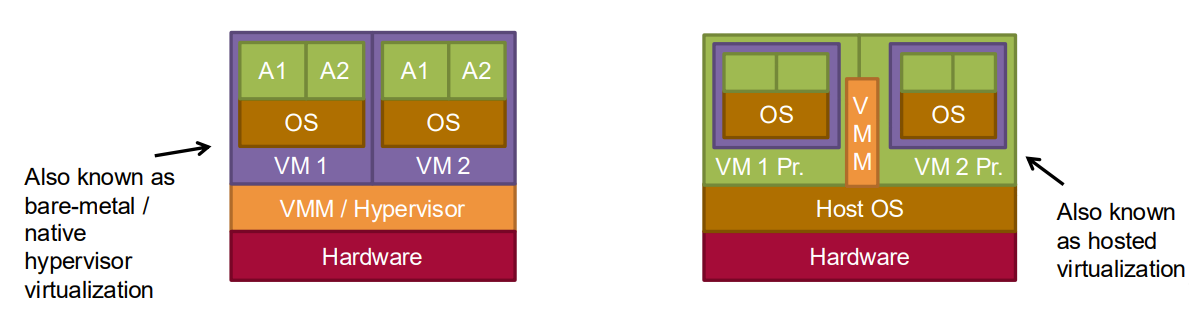
Hypervisor (Virtual Machine Monitor)
The hypervisor is the software layer that enables the creation and management of virtual machines:
Type 1 Hypervisors: Run directly on hardware (bare-metal)
Examples: VMware ESXi, Microsoft Hyper-V, Xen, KVM
More efficient, commonly used in data centers and cloud environments
Type 2 Hypervisors: Run on top of a host operating system
Common for desktop virtualization and development environments
Guest Operating System
The operating system that runs inside the VM, which can be different from the host system.
Virtual Hardware
Virtualized components presented to the VM:
Virtual CPUs (vCPUs)
Virtual RAM
Virtual Disks
Virtual Network Interfaces
Virtual I/O devices
VM Images
Templates containing the VM configuration and virtual disk content:
Pre-configured operating systems and applications
Stored as files on the host system
Can be used to rapidly deploy new VMs
Virtualizability
For a system to be efficiently virtualized, certain conditions must be met. Popek and Goldberg’s theorem states:
“A virtual machine monitor may be constructed if the set of sensitive instructions for that computer is a subset of the set of privileged instructions.”
Where:
Privileged instructions: Instructions that can only execute in system mode
Sensitive instructions: Instructions that could affect system resources or behave differently based on system state
This theorem is the foundation for understanding the challenges in virtualizing architectures like x86.
Virtualization Approaches
Different approaches to virtualization have emerged to address architectural challenges:
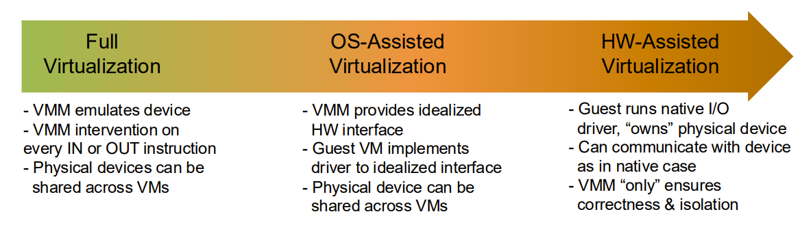
Full Virtualization: Guest OS runs unmodified, unaware it’s being virtualized
May require techniques like binary translation to handle non-virtualizable instructions
Full virtualization is a virtualization technique where the virtual machine simulates enough hardware to allow an unmodified guest operating system to run in isolation. In full virtualization, the guest OS is completely unaware that it is being virtualized and requires no modifications.
Key Characteristics
Guest operating system runs unmodified
No modifications to the guest OS source code or binaries
Complete isolation between guest and host
Higher resource overhead compared to other virtualization techniques
Challenges with x86 Architecture
The x86 architecture presented significant challenges for full virtualization because it doesn’t satisfy the Popek and Goldberg’s Theorem requirements:
Some sensitive instructions don’t trap when executed in user mode
These “critical instructions” prevent traditional trap-and-emulate virtualization
Binary Translation
To overcome these challenges, virtualization systems like VMware developed binary translation:
How Binary Translation Works
Dynamic Code Analysis:
The VMM analyzes the guest OS code at runtime
Identifies sequences of instructions (translation units)
Looks for critical instructions in these units
Code Replacement:
Critical instructions are replaced with alternative code that:
Achieves the same functionality
Allows the VMM to maintain control
May include explicit calls to the VMM
Translation Cache:
Modified code blocks are stored in a translation cache
Frequently executed code benefits from this caching
Translation is done lazily (only when needed)
Direct Execution:
Non-critical, unprivileged instructions run directly on the CPU
This minimizes performance overhead for regular code
Memory Management in Full Virtualization
Shadow Page Tables
To handle memory virtualization, full virtualization uses shadow page tables:
Guest OS maintains its own page tables (logical to “physical” mapping)
VMM maintains shadow page tables (logical to actual physical mapping)
When guest modifies its page tables, operations trap to the VMM
VMM updates shadow page tables accordingly
The hardware MMU uses the shadow page tables for actual translation
This creates two levels of address translation:
Guest virtual address → Guest physical address
Guest physical address → Host physical address
Shadow page tables combine these translations for efficiency.
I/O Virtualization in Full Virtualization
Several approaches exist for I/O virtualization:
Device Emulation:
VMM presents virtual devices to the guest
Common devices emulated include disk controllers, network cards, etc.
Guest uses standard drivers for these virtual devices
Device Driver Interception:
VMM intercepts calls to virtual device drivers
Redirects to corresponding physical devices
Device Passthrough:
Direct assignment of physical devices to VMs
Requires hardware support (IOMMU)
Offers better performance but limits device sharing
Performance Implications
Full virtualization has performance implications:
CPU overhead for binary translation
Memory overhead for shadow page tables
I/O performance degradation due to interception and emulation
High context switching overhead for privileged operations
Examples of Full Virtualization
VMware Workstation
Oracle VirtualBox
Microsoft Virtual PC
QEMU (when used without KVM)
Advantages and Disadvantages
Advantages
No modification to guest OS required
Can run any operating system designed for the same architecture
Complete isolation between VMs
Disadvantages
Performance overhead, especially for I/O operations
OS-assisted virtualization, also known as paravirtualization, is a virtualization technique where the guest operating system is modified to be aware that it is running in a virtualized environment. This approach allows the guest OS to cooperate with the hypervisor to achieve better performance than full virtualization, especially on architectures that don’t perfectly satisfy Popek and Goldberg’s Theorem.
Key Concept
The fundamental idea of OS-assisted virtualization is to:
Make the guest OS aware that it is being virtualized and modify it to directly communicate with the hypervisor, avoiding the need for complex techniques like binary translation or hardware extensions.
How OS-Assisted Virtualization Works
The guest OS is modified to replace non-virtualizable instructions with explicit calls to the hypervisor (hypercalls)
The guest OS is aware it doesn’t have direct access to physical hardware
The hypervisor provides an API that the modified guest OS uses for privileged operations
The guest still maintains its device drivers, memory management, and process scheduling, but in coordination with the hypervisor
Xen: A Classic Example
Xen is the most well-known example of OS-assisted virtualization:
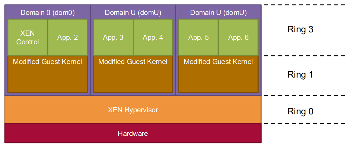
Xen Architecture
Hypervisor: A thin layer running directly on hardware (Type 1)
Domain 0 (dom0): Privileged guest for control and management
Domain U (domU): Unprivileged guest domains with Xen-aware OS
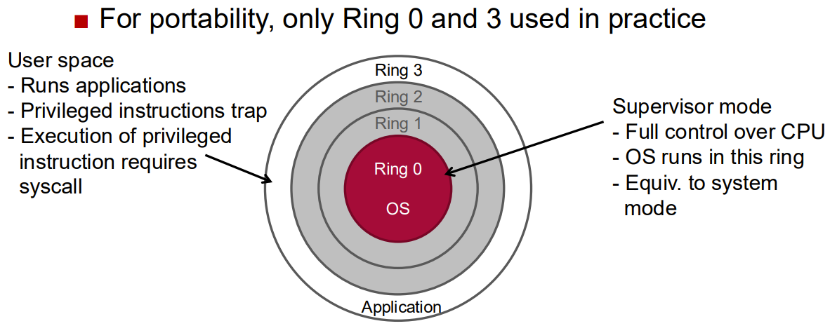
Xen uses a ring structure for privileges:
Hypervisor runs in Ring 0 (most privileged)
Guest OS kernels run in Ring 1
Guest applications run in Ring 3 (least privileged)
CPU Virtualization in Xen
Guest OS is modified to run in Ring 1 instead of Ring 0
Critical instructions are replaced with hypercalls
Hypercalls are explicit calls from the guest OS to the hypervisor
System calls from applications to the guest OS can sometimes bypass the hypervisor for better performance
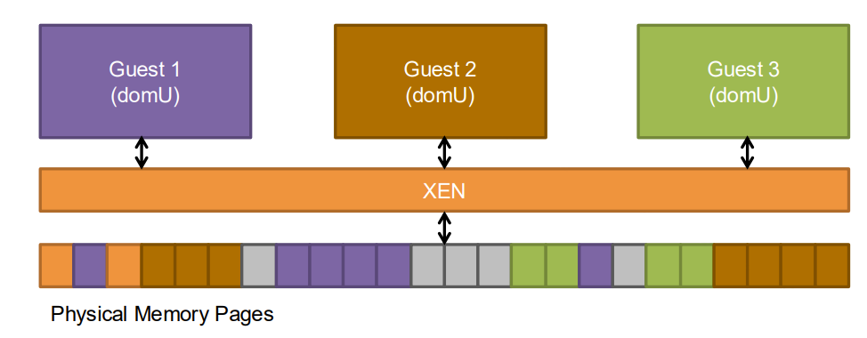
Memory Management in Xen
Xen’s approach to memory management is distinctive:
Physical memory is statically partitioned among domains at creation time
Each domain is aware of its physical memory allocation
Domains maintain their own page tables, validated by the hypervisor
The guest page tables are used directly by the hardware MMU
Updates to page tables require hypervisor validation to ensure isolation
Hardware-assisted virtualization refers to virtualization techniques that leverage special processor features designed specifically to support virtual machines. These hardware extensions were introduced to overcome the limitations of x86 architecture that made it difficult to efficiently virtualize according to Popek and Goldberg’s Theorem.
Background
The classic x86 architecture contained about 17 “critical instructions” (sensitive but not privileged) that prevented efficient virtualization. To address this issue, both Intel and AMD independently developed hardware virtualization extensions:
Intel VT-x (Intel Virtualization Technology for x86)
AMD-V (AMD Virtualization)
These technologies were introduced in 2005-2006 and have since evolved to include more advanced features.
IA-32:
Core Concepts
CPU Virtualization Extensions
The primary innovation in hardware-assisted virtualization is the introduction of new CPU modes:
Root Mode: Where the VMM/hypervisor runs
Non-root Mode: Where guest OSes run (called “guest mode”)
This creates a higher privilege level for the hypervisor than even Ring 0, allowing guest OSes to run in their expected privilege rings while still being controlled by the hypervisor.
The transitions between these modes are:
VM Entry: Transition from root mode to non-root mode
VM Exit: Transition from non-root mode to root mode
VMM Control Structures
The CPU maintains control structures for each virtual machine:
Intel VMCS (Virtual Machine Control Structure)
AMD VMCB (Virtual Machine Control Block)
These structures contain:
Guest state (register values, control registers, etc.)
Host state (to be restored on VM Exit)
Execution controls (what events cause VM Exits)
Exit information (why a VM Exit occurred)
Key Mechanisms
Control Registers:
Special CPU registers that determine VM Exit conditions
Allow fine-grained control over which events trap to the hypervisor
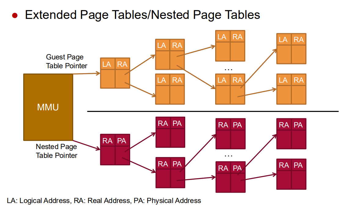
Extended Page Tables / Nested Page Tables:
Intel EPT / AMD NPT
Hardware support for two-level address translation
Eliminates shadow page table overhead
Tagged TLBs:
Associate TLB entries with specific address spaces
Avoid TLB flushes on context switches between VMs
IOMMU (I/O Memory Management Unit):
Intel VT-d / AMD-Vi
Provides DMA remapping and interrupt remapping
Enables safe direct device assignment to VMs
Memory Virtualization Extensions
One significant advancement in hardware-assisted virtualization is the support for nested paging:
Virtual Machines (VMs) and containers are both virtualization technologies that enable software to run in isolated environments, but they differ significantly in their architecture, resource usage, performance characteristics, and use cases.
Architectural Differences
Virtual Machines
Level of Virtualization: Hardware-level virtualization
Containers are a lightweight form of virtualization that package an application and its dependencies into a standardized unit for software development and deployment. Unlike virtual machines, containers virtualize at the operating system level rather than at the hardware level.
Definition
Containers, also known as OS-level virtualization, provide isolated environments for running application processes within a shared operating system kernel. They encapsulate an application with its runtime, system tools, libraries, and settings needed to run, ensuring consistency across different environments.
Resource Utilization: Containers share the host OS kernel, making them more lightweight
Isolation Level: Containers isolate at the process level; VMs isolate at the hardware level
Startup Time: Containers start in seconds; VMs typically take minutes
Image Size: Container images are typically megabytes; VM images are gigabytes
Portability: Containers provide consistent runtime regardless of underlying infrastructure
Container Images
A container image is a lightweight, standalone, executable package that includes everything needed to run an application:
Application code
Runtime environment
System libraries
Default settings
Images are built in layers, which are cached and reused across containers to optimize storage and transfer efficiency.
Container Instances
A container instance is a running copy of a container image. Multiple instances can run from the same image simultaneously, each with its own isolated environment.
Evolution of Containerization
Early Isolation Mechanisms
chroot (1979): The first UNIX mechanism for isolating a process’s file system view
FreeBSD Jails (2000): Extended isolation to include processes, networking, and users
Solaris Zones (2004): Similar isolation capabilities for Solaris
Modern Container Technologies
LXC (2008): Linux Containers using kernel containment features
Docker (2013): Made containers accessible with simplified tooling and images
rkt/Rocket (2014): Alternative container runtime with focus on security
Podman (2018): Daemonless container engine compatible with Docker
The Linux kernel includes several mechanisms that enable process isolation and resource control, which collectively form the foundation for container technologies. These containment features allow for efficient OS-level virtualization without the overhead of full system virtualization.
Core Containment Mechanisms
1. chroot
The chroot system call, introduced in 1979 in UNIX Version 7, is the oldest isolation mechanism and a precursor to modern containerization:
Changes the apparent root directory for a process and its children
Limits a process’s view of the file system
Isolates file system access but doesn’t provide complete isolation
Used primarily for security and creating isolated build environments
# Example: Changing root directory for a processsudo chroot /path/to/new/root command
2. Namespaces
Namespaces partition kernel resources so that one set of processes sees one set of resources while another set of processes sees a different set. Linux includes several types of namespaces:
PID Namespace
Isolates process IDs
Each namespace has its own process numbering, starting at PID 1
Processes in a namespace can only see other processes in the same namespace
Enables container restart without affecting other containers
Network Namespace
Isolates network resources
Each namespace has its own:
Network interfaces
IP addresses
Routing tables
Firewall rules
Port numbers
Mount Namespace
Isolates filesystem mount points
Each namespace has its own view of the filesystem hierarchy
Changes to mounts in one namespace don’t affect others
Fundamental for container filesystem isolation
UTS Namespace
Isolates hostname and domain name
Allows each container to have its own hostname
Named after UNIX Time-sharing System
IPC Namespace
Isolates Inter-Process Communication resources
Isolates System V IPC objects and POSIX message queues
Prevents processes in different namespaces from communicating via IPC
User Namespace
Isolates user and group IDs
A process can have root privileges within its namespace while having non-root privileges outside
Enhances container security
Time Namespace
Introduced in newer kernel versions
Allows containers to have their own system time
3. Control Groups (cgroups)
Control groups, or cgroups, provide mechanisms for:
Cgroups organize processes hierarchically and distribute system resources along this hierarchy:
Cgroup Subsystems (Controllers)
cpu: Limits CPU usage
memory: Limits memory usage and reports memory resource usage
blkio: Limits block device I/O
devices: Controls access to devices
net_cls: Tags network packets for traffic control
freezer: Suspends and resumes processes
pids: Limits process creation
4. Capabilities
Linux capabilities divide the privileges traditionally associated with the root user into distinct units that can be independently enabled or disabled:
Allows for fine-grained control over privileged operations
Reduces the security risks of running processes as root
Examples of capabilities:
CAP_NET_ADMIN: Configure networks
CAP_SYS_ADMIN: Perform system administration operations
CAP_CHOWN: Change file ownership
5. Security Modules
Linux includes several security modules that can enhance container isolation:
SELinux (Security-Enhanced Linux)
Provides Mandatory Access Control (MAC)
Defines security policies that constrain processes
Labels files, processes, and resources, controlling interactions based on these labels
AppArmor
Path-based access control
Restricts programs’ capabilities using profiles
Simpler to configure than SELinux, used by default in Ubuntu
Seccomp (Secure Computing Mode)
Filters system calls available to a process
Prevents processes from making unauthorized system calls
Can be used with a whitelist or blacklist approach to control system call access
# Example: Activating seccomp profile in Dockerdocker run --security-opt seccomp=/path/to/profile.json image_name
Implementation in Container Technologies
These Linux kernel features are used by container runtimes in various combinations:
LXC: Utilizes all these features directly with a focus on system containers
Docker: Builds upon these features with additional tooling and image management
Podman: Similar to Docker but with a focus on rootless containers using user namespaces
Kubernetes/CRI-O: Uses these features via container runtimes like containerd or CRI-O
Limitations and Considerations
Despite these isolation mechanisms, some limitations remain:
Kernel Sharing: All containers share the host kernel, which means:
Kernel vulnerabilities affect all containers
Containers cannot run a different OS kernel than the host
Resource Contention: Without proper cgroup configurations, noisy neighbors can still impact performance
Security Concerns: Container escape vulnerabilities can potentially compromise the host
Docker is a leading containerization platform that simplifies the process of creating, deploying, and running applications in containers. Released in 2013, Docker revolutionized application deployment by making container technology accessible and standardized.
Core Concepts
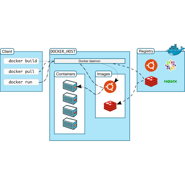
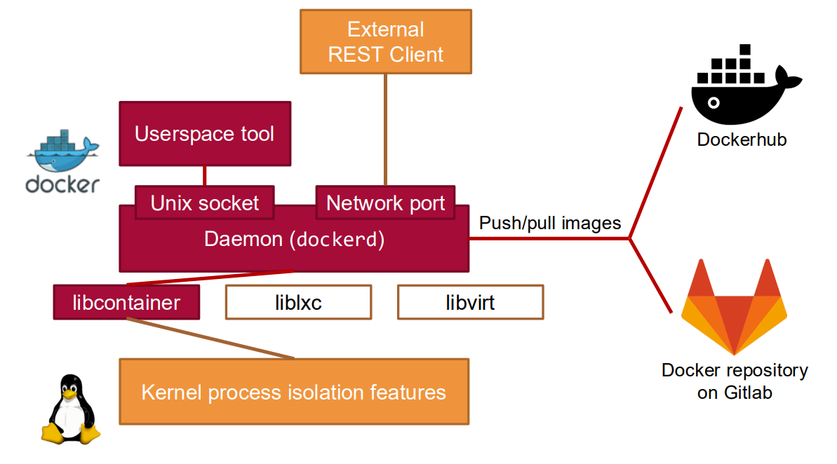
Docker Architecture
Docker uses a client-server architecture consisting of:
Docker Client: The primary user interface to Docker
Docker Daemon (dockerd): A persistent process that manages Docker containers
Docker Registry: A repository for Docker images (e.g., Docker Hub)
Docker Components
Docker Engine
The Docker Engine is the core of Docker, comprising:
Docker daemon: Runs in the background and handles container operations
REST API: Provides an interface for the client to communicate with the daemon
Command-line interface (CLI): The user interface for Docker commands
Docker Images
A Docker image is a read-only template containing a set of instructions for creating a Docker container:
Built in layers, with each layer representing a set of filesystem changes
Defined in a Dockerfile
Stored in a registry (e.g., Docker Hub or private registry)
Immutable: once built, the image doesn’t change
Docker Containers
A container is a runnable instance of an image:
Isolated environment for running applications
Contains everything needed to run the application (code, runtime, libraries, etc.)
Shares the host OS kernel but is isolated at the process level
Docker Image Format
Docker images use a layered architecture that provides several benefits:
Efficient storage: Layers are cached and reused across images
Faster transfers: Only new or modified layers need to be transferred
Version control: Each layer represents a change, enabling versioning
Image Layers
An image consists of multiple read-only layers, each representing a set of filesystem changes:
Base layer: Usually a minimal OS distribution
Additional layers: Each layer adds, modifies, or removes files from the previous layer
Container layer: When a container runs, a writable layer is added on top
Content Addressable Storage
Docker uses content-addressable storage for images:
Each layer is identified by a hash of its contents
Ensures image integrity and enables deduplication
Allows deterministic builds and reproducibility
Dockerfiles
A Dockerfile is a text file containing instructions for building a Docker image:
COPY/ADD: Copies files from the build context into the image
WORKDIR: Sets the working directory
ENV: Sets environment variables
EXPOSE: Documents the ports the container will listen on
VOLUME: Creates a mount point for external volumes
ENTRYPOINT: Configures the executable to run when the container starts
CMD: Provides default arguments for the ENTRYPOINT
Docker Commands
Basic Commands
# Build an imagedocker build -t myapp:1.0 .# Run a containerdocker run -d -p 8080:80 myapp:1.0# List running containersdocker ps# Stop a containerdocker stop container_id# Remove a containerdocker rm container_id# List imagesdocker images# Remove an imagedocker rmi image_id
Advanced Commands
# Inspect a containerdocker inspect container_id# View container logsdocker logs container_id# Execute a command in a running containerdocker exec -it container_id bash# Create a new image from a containerdocker commit container_id new_image_name:tag# Push an image to a registrydocker push username/repository:tag
Docker Compose
Docker Compose is a tool for defining and running multi-container Docker applications:
Uses a YAML file to configure application services
Enables managing multiple containers as a single application
Simplifies development and testing workflows
Example docker-compose.yml
version: '3'services: web: build: ./web ports: - "8080:80" depends_on: - db db: image: postgres:13 volumes: - postgres_data:/var/lib/postgresql/data environment: POSTGRES_PASSWORD: example POSTGRES_USER: user POSTGRES_DB: mydbvolumes: postgres_data:
Docker Networking
Docker provides several network drivers for container communication:
bridge: Default network driver, allows containers on the same host to communicate
Container orchestration automates the deployment, management, scaling, and networking of containers. As applications grow in complexity and scale, manually managing individual containers becomes impractical, making orchestration essential for production container deployments.
What is Container Orchestration?
Container orchestration refers to the automated arrangement, coordination, and management of containers. It handles:
Provisioning and deployment of containers
Resource allocation
Load balancing across multiple hosts
Health monitoring and automatic healing
Scaling containers up or down based on demand
Service discovery and networking
Rolling updates and rollbacks
Why Container Orchestration is Needed
Challenges of Manual Container Management
Scale: Managing hundreds or thousands of containers manually is impossible
Complexity: Multi-container applications have complex dependencies
Reliability: Manual intervention increases the risk of errors
Resource Utilization: Optimal placement of containers requires sophisticated algorithms
High Availability: Fault tolerance requires automated monitoring and recovery
Benefits of Container Orchestration
Automated Operations: Reduces manual intervention and human error
Optimal Resource Usage: Intelligent scheduling of containers
Self-healing: Automatic recovery from failures
Scalability: Easy horizontal scaling
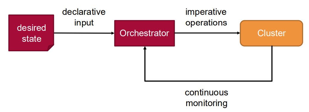
Declarative Configuration: Define desired state rather than imperative steps
Service Discovery: Automatic linking of interconnected components
Load Balancing: Distribution of traffic across container instances
Rolling Updates: Zero-downtime deployments
Core Concepts in Container Orchestration
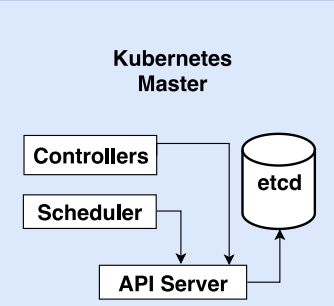
Master
Collection of processes managing the cluster state on
a single node of the cluster
Controllers, e.g. replication and
scaling controllers
Scheduler: places pods based on
resource requirements, hardware
and software constraints, data locality, deadlines…
etcd: reliable distributed key-value store, used for the
cluster state
Cluster
A collection of host machines (physical or virtual) that run containerized applications managed by the orchestration system.
Node
An individual machine (physical or virtual) in the cluster that can run containers.
Container
The smallest deployable unit, running a single application or process.
Pod
In Kubernetes, a group of one or more containers that share storage and network resources and a specification for how to run the containers.
Service
An abstraction that defines a logical set of pods and a policy to access them, often used for load balancing and service discovery.
Desired State
The specification of how many instances should be running, what version they should be, and how they should be configured.
Reconciliation Loop
The process by which the orchestration system continuously works to make the current state match the desired state.
Key Features of Orchestration Platforms
Scheduling
Placement Strategies: Determining which node should run each container
Affinity/Anti-affinity Rules: Controlling which containers should or shouldn’t run together
Resource Constraints: Considering CPU, memory, and storage requirements
Kubernetes (often abbreviated as K8s) is an open-source container orchestration platform designed to automate deploying, scaling, and managing containerized applications. Originally developed by Google and now maintained by the Cloud Native Computing Foundation (CNCF), Kubernetes has become the de facto standard for container orchestration.
History and Background
Origin: Developed by Google based on their internal system called Borg
Release: Open-sourced in 2014
Name: Greek for “helmsman” or “pilot” (hence the ship’s wheel logo)
CNCF: Became the first graduated project of the Cloud Native Computing Foundation in 2018
Core Concepts
Kubernetes Architecture
Kubernetes follows a master-worker (also called control plane and node) architecture:
Control Plane Components
API Server: Front-end for the Kubernetes control plane, exposing the Kubernetes API
etcd: Consistent and highly-available key-value store for all cluster data
Scheduler: Watches for newly created pods with no assigned node and selects nodes for them to run on
Controller Manager: Runs controller processes that regulate the state of the cluster
Cloud Controller Manager: Links the cluster to cloud provider APIs
Node Components
Kubelet: An agent that runs on each node, ensuring containers are running in a pod
Kube-proxy: Network proxy that maintains network rules on nodes
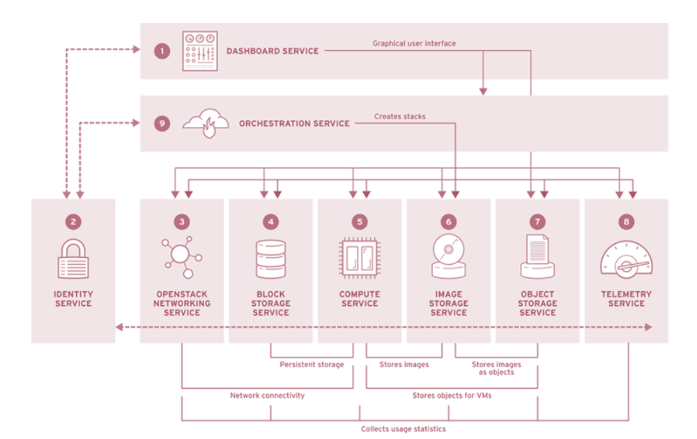
Cloud operating systems are software platforms that manage large pools of compute, storage, and networking resources in a data center, providing interfaces for both administrators and users. They serve as the foundation for Infrastructure as a Service (IaaS) cloud offerings, abstracting underlying hardware complexities and enabling the provisioning of virtual resources.
Purpose and Function
Cloud operating systems serve several key functions:
Resource Virtualization: Abstract physical hardware into virtual resources
Resource Management: Allocate and track usage of compute, storage, and networking resources
Multi-tenancy: Enable secure sharing of physical infrastructure among multiple users
User Interface: Provide dashboards and APIs for cloud administrators and end users
Automation: Enable programmatic control over infrastructure components
Key Components and Features
Core Functionality
Compute Management: Creation and management of virtual machines
Storage Management: Provisioning of virtual disks and object storage
Infrastructure as Code (IaC) is the practice of managing and provisioning computing infrastructure through machine-readable definition files rather than physical hardware configuration or interactive configuration tools. It enables infrastructure to be defined, versioned, and deployed in a repeatable, consistent manner.
Core Concepts
Definition and Principles
Infrastructure as Code treats infrastructure configuration as software code that can be:
Written: Defined in text files with specific syntax or domain-specific languages
Versioned: Tracked in version control systems (Git, SVN, etc.)
Tested: Validated through automated testing
Deployed: Applied automatically to create or modify infrastructure
Reused: Shared and composed to build complex environments
Key Benefits
Consistency: Eliminates configuration drift and “snowflake servers”
Version Control: Tracks changes and enables rollbacks
Documentation: Self-documenting infrastructure through code
Collaboration: Enables team-based infrastructure development
Risk Reduction: Automated deployments reduce human error
Cost Efficiency: Optimizes resource usage through precise specifications
Challenges Addressed by IaC
Configuration Drift
Configuration drift occurs when systems’ actual configurations diverge from their documented or expected states due to manual changes, ad-hoc fixes, or inconsistent updates. IaC addresses this by:
Defining a single source of truth for infrastructure
Enabling detection of unauthorized changes
Facilitating reconciliation between actual and desired states
Snowflake Servers
Snowflake servers are unique, manually configured servers that:
Have undocumented configurations
Cannot be easily replicated
Represent significant operational risk
Are difficult to maintain and update
IaC replaces snowflake servers with reproducible, consistent infrastructure.
Manual Configuration Problems
Manual configuration processes lead to:
Inconsistent environments
Error-prone deployments
Poor documentation
Slow provisioning times
Difficult recovery from failures
Approaches to Infrastructure as Code
Declarative vs. Imperative
Declarative Approach
Describes the desired end state of the infrastructure
System determines how to achieve that state
Idempotent: repeated applications yield the same result
Virtual machine (VM) management encompasses various operations for creating, monitoring, maintaining, and migrating virtual machines in cloud environments. Effective VM management is crucial for optimizing resource usage, ensuring high availability, and maintaining operational efficiency in cloud infrastructures.
VM Lifecycle Management
VM Creation and Deployment
The process of creating and deploying VMs involves:
VM Image Selection: Choosing a base image with the required OS and software
Resource Allocation: Assigning CPU, memory, storage, and network resources
Configuration: Setting VM parameters (name, network, storage paths)
Provisioning: Creating the VM instance from the configuration
Post-deployment Configuration: Additional setup after VM is running
VM Maintenance Operations
Common VM maintenance operations include:
Starting/Stopping: Powering VMs on or off
Pausing/Resuming: Temporarily suspending VM execution
Patching/Updating: Applying OS or software updates
Backup/Restore: Creating and using VM backups
Monitoring: Tracking performance and health metrics
VM Snapshots
VM snapshots capture the state of a virtual machine at a specific point in time:
Full Snapshots: Capture entire VM state, including memory
Disk-only Snapshots: Capture only disk state
Virtual Snapshots: Use copy-on-write to reduce storage overhead
Snapshot Trees: Create hierarchical relationships between snapshots
Use Cases for Snapshots:
Creating system restore points before major changes
Testing software updates with easy rollback
Backup and recovery
VM cloning and templating
Snapshot Limitations:
Performance impact during creation and while active
Storage space consumption
Not a substitute for proper backup strategies
Potential consistency issues for applications
VM Migration
VM migration is the process of moving a virtual machine from one physical host to another or from one storage location to another. This capability is essential for resource optimization, hardware maintenance, and fault tolerance.
Types of VM Migration
Based on VM State:
Cold Migration
VM is powered off before migration
Complete VM files are copied to the destination
VM is started on the destination host
No downtime requirement, but service interruption
Warm Migration
VM is suspended (state saved to disk)
VM files and state are copied to the destination
VM is resumed on the destination
Brief service interruption
Live Migration (Hot Migration)
VM continues running during migration
State is iteratively copied while tracking changes
Final brief switchover when difference is minimal
Minimal or no perceptible downtime
Based on Migration Scope:
Compute Migration: Moving VM execution
Storage Migration: Moving VM disk files
Combined Migration: Moving both compute and storage
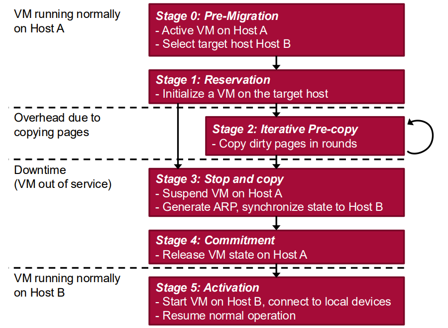
Live Migration Process
Live migration typically follows these steps:
Pre-migration:
Select source and destination hosts
Verify compatibility and resource availability
Establish migration channel
Reservation:
Reserve resources on the destination host
Create container for the VM on destination
Iterative Pre-copy:
Initial copy of memory pages
Iterative copying of modified (dirty) pages
Continue until rate of page changes stabilizes or threshold reached
Stop-and-Copy Phase:
Brief suspension of VM on source
Copy remaining dirty pages
Synchronize final state
Commitment:
Confirm successful copy to destination
Release resources on source
Activation:
Resume VM execution on destination
Update network routing/addressing
Resume normal operation
Live Migration Techniques and Technologies
Memory Migration Strategies
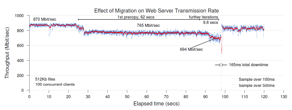
Pre-copy Approach (most common):
VM continues running on source during initial copying
Memory pages modified during copy are tracked and re-copied
Multiple rounds of copying dirty pages
VM paused briefly for final synchronization
Post-copy Approach:
Minimal VM state transferred initially
VM starts running on destination immediately
Memory pages fetched from source on demand
Background process copies remaining pages
Hybrid Approaches:
Combine pre-copy and post-copy techniques
Adaptively choose strategy based on workload
Network Migration
For successful VM migration, network connections must be preserved:
DevOps is a set of practices that combines software development (Dev) and IT operations (Ops) with the goal of shortening the development lifecycle and delivering high-quality software continuously. Continuous Integration and Continuous Delivery/Deployment (CI/CD) are core practices within the DevOps methodology, providing automation for building, testing, and deploying software.
DevOps Overview
Definition and Philosophy
DevOps represents a cultural shift in how software development and operations teams collaborate:
Cultural Integration: Breaking down silos between development and operations teams
A distributed system can be defined in several ways:
Tanenbaum and van Steen: “A collection of independent computers that appears to its users as a single coherent system”
Coulouris, Dollimore and Kindberg: “One in which hardware or software components located at networked computers communicate and coordinate their actions only by passing messages”
Lamport: “One that stops you getting work done when a machine you’ve never even heard of crashes”
Motivations for Distributed Systems
Geographic Distribution: Resources and users are naturally distributed
Example: Banking services accessible from different locations while data is centrally stored
Modern cloud architectures are built on several key concepts that address the challenges of building large-scale, distributed, and reliable systems. This note provides an overview of the architectural approaches used in modern cloud systems.
Architectural Foundations
Modern cloud architectures are founded on two fundamental pillars:
Vertical integration - Enhancing capabilities within individual tiers/services
Horizontal scaling - Using multiple commodity computers working together
These pillars have led to significant shifts away from monolithic application architectures toward more distributed approaches.
Architectural Concepts
Layering
Definition: Partitioning services vertically into layers
Lower layers provide services to higher ones
Higher layers unaware of underlying implementation details
Low inter-layer dependency
Examples:
Network protocol stacks (OSI model)
Operating systems (kernel, drivers, libraries, GUI)
Games (engine, logic, AI, UI)
Advantages:
Abstraction
Reusability
Loose coupling
Isolated management and testing
Supports software evolution
Tiering
Definition: Mapping the organization of and within a layer to physical or virtual devices
Implies physical location considerations
Complements layering
Classic Architectures:
2-tier (client-server): Split layers between client and server
3-tier: User Interface, Application Logic, Data tiers
n-tier/multi-tier: Further division (e.g., microservices)
Advantages:
Scalability
Availability
Flexibility
Easier management
Monolith vs. Distributed Architecture
Monolithic Architecture
Definition: A single, tightly coupled block of code with all application components
Advantages:
Simple to develop and deploy
Easy to test and debug in early stages
Disadvantages:
Increasing complexity as application grows
Difficult to scale individual components
Limited agility with slow and risky deployments
Technology lock-in
Distributed Architecture
Definition: Application divided into loosely coupled components running on separate servers
Advantages:
Independent scaling of components
Fault isolation
Technology diversity
Better maintainability
Disadvantages:
Network communication overhead
More complex to manage
Distributed debugging challenges
Practical Application Guidelines
When designing cloud architectures:
Foundation matters: Just as buildings need proper foundations, cloud architectures require robust infrastructure layers
Consider scalability & modularity: Employ modular techniques for easier expansion and modification
Focus on resource efficiency: Implement auto-scaling, serverless approaches, and efficient resource allocation
Plan for evolution: Design systems that can adapt to new technologies while maintaining stability
Modern Cloud Architectures - Redundancy
Redundancy is a key design principle in modern cloud architectures that improves fault tolerance, availability, and performance.
Why Use Redundancy?
Performance: Distribute workload across multiple replicas to improve response time
Error Detection: Compare results when replicas disagree
Error Recovery: Switch to backup resources when primary fails
Fault Tolerance: System continues functioning despite component failures
Importance of Fault Models
The effectiveness of redundancy depends on how individual replicas fail:
For independent crash faults, the availability of a system with n replicas is:
Availability = 1-p^n
Where p is the probability of individual failure
Example: 5 servers each with 90% uptime → overall availability = 1-(0.10)^5 = 99.999%
This only holds if failures are truly independent, which requires consideration of common failure modes.
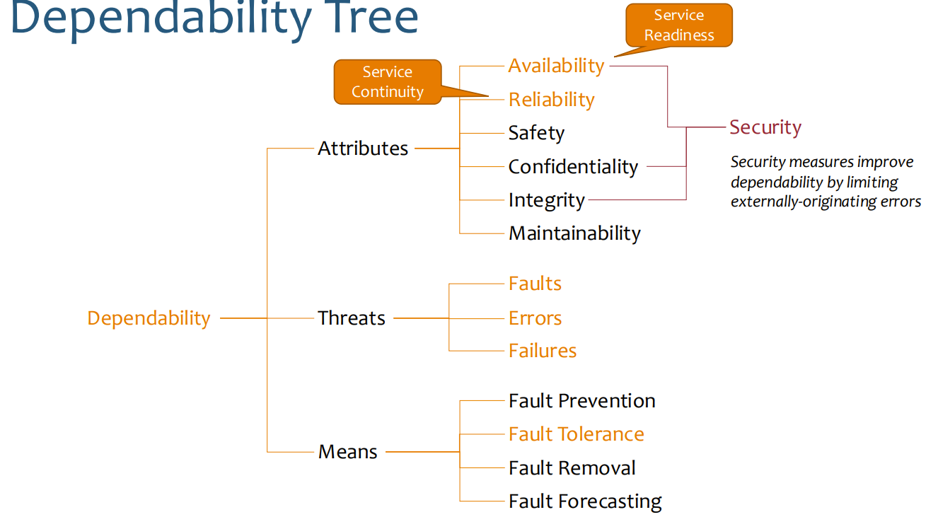
Fault tolerance is the ability of a system to continue operating properly in the event of the failure of one or more of its components. It’s a key attribute for achieving high availability and reliability in distributed systems, especially in cloud environments where component failures are expected rather than exceptional.
Core Concepts
Faults vs. Failures
It’s important to distinguish between faults and failures:
Fault: A defect in a system component that can lead to an incorrect state
Error: The manifestation of a fault that causes a deviation from correctness
Failure: When a system deviates from its specified behavior due to errors
Fault tolerance aims to prevent faults from becoming system failures.
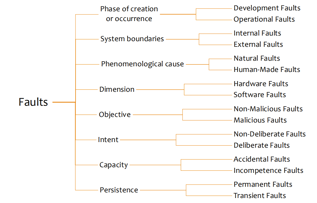
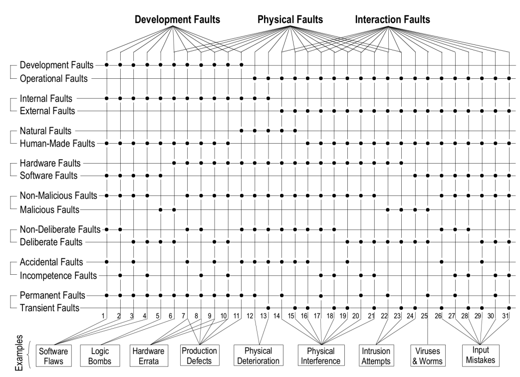
Types of Faults
Faults can be categorized in several ways:
By Duration
Transient Faults: Occur once and disappear (e.g., network packet loss)
Intermittent Faults: Occur occasionally and unpredictably (e.g., connection timeouts)
Permanent Faults: Persist until the faulty component is repaired (e.g., hardware failures)
Load balancing is the process of distributing network traffic across multiple servers to ensure no single server bears too much demand. By spreading the workload, load balancing improves application responsiveness and availability, while preventing server overload.
Core Concepts
Purpose of Load Balancing
Load balancing serves several critical functions:
Scalability: Handling growing workloads by adding more servers
Availability: Ensuring service continuity even if some servers fail
Reliability: Redirecting traffic away from failed or degraded servers
Performance: Optimizing response times and resource utilization
Efficiency: Maximizing throughput and minimizing latency
Load Balancer Placement
Load balancers can operate at various points in the infrastructure:
Client-Side: Load balancing decisions made by clients (e.g., DNS-based)
Server-Side: Dedicated load balancer in front of server pool
Network-Based: Load balancing within the network infrastructure
Global: Geographic distribution of traffic across multiple data centers
Load Balancing Algorithms
Static Algorithms
Static algorithms don’t consider the real-time state of servers:
Round Robin
Each request is assigned to servers in circular order
Simple and fair but doesn’t account for server capacity or load
Variants: Weighted Round Robin gives some servers higher priority
IP Hash
Uses the client’s IP address to determine which server receives the request
Ensures the same client always reaches the same server (session affinity)
Useful for stateful applications where session persistence matters
Dynamic Algorithms
Dynamic algorithms adapt based on server conditions:
Least Connections
Directs traffic to the server with the fewest active connections
Assumes connections require roughly equal processing time
Variants: Weighted Least Connections accounts for different server capacities
Least Response Time
Sends requests to the server with the lowest response time
Better distributes load based on actual server performance
More CPU-intensive for the load balancer to implement
Resource-Based
Distributes load based on CPU usage, memory, bandwidth, or other metrics
Requires monitoring agents on servers to report resource utilization
Cloud computing offers different service models, each providing a different level of abstraction and management. These models define what resources are managed by the provider versus the customer.
Traditional Service Models
Infrastructure as a Service (IaaS)
Definition: Provider provisions processing, storage, network, and other fundamental computing resources where the customer can deploy and run arbitrary software, including operating systems and applications.
Customer manages:
Operating systems
Middleware
Applications
Data
Runtime environments
Provider manages:
Servers and storage
Networking
Virtualization
Data center infrastructure
Key characteristics:
Most flexible cloud service model
Customer has maximum control over infrastructure configuration
Requires the most technical expertise to manage
Examples:
Amazon EC2
Google Compute Engine
Microsoft Azure VMs
OpenStack
Platform as a Service (PaaS)
Definition: Customer deploys applications onto cloud infrastructure using programming languages, libraries, services, and tools supported by the provider.
Customer manages:
Applications
Data
Some configuration settings
Provider manages:
Operating systems
Middleware
Runtime
Servers and storage
Networking
Data center infrastructure
Key characteristics:
Reduces complexity of infrastructure management
Accelerates application deployment
Often includes development tools and services
Less control compared to IaaS
Examples:
Heroku
Google App Engine
Microsoft Azure App Service
AWS Elastic Beanstalk
Software as a Service (SaaS)
Definition: Provider delivers applications running on cloud infrastructure accessible through various client devices, typically via a web browser.
Customer manages:
Minimal application configuration
Data (to some extent)
Provider manages:
Everything including the application itself
All underlying infrastructure and software
Key characteristics:
Minimal management required from customer
Typically subscription-based
Immediate usability
Limited customization
Examples:
Microsoft Office 365
Google Workspace
Salesforce
Dropbox
IaaS in Detail
How IaaS Works
Customer requests VMs with specific configurations (CPU, RAM, storage)
Provider matches request against available data center machines
VMs are provisioned on physical hosts with requested resources
Customer accesses and manages VMs through provided interfaces
Resource Allocation
CPU allocation: Either pinned to specific cores or scheduled by the hypervisor
Memory allocation: Usually strictly partitioned between VMs
Storage: Allocated based on requested volume sizes
Network resources: Shared among VMs with quality of service controls
IaaS APIs
IaaS providers offer APIs for programmatic control of resources:
Create, start, stop, clone operations
Monitoring capabilities
Pricing information access
Resource management
Benefits:
Flexibility through code-based infrastructure control
Automation of provisioning and management
Integration with other tools and systems
IaaS Pricing Models
Typically based on a combination of:
VM instance type/size
Duration of usage (per hour/minute)
Storage consumption
Network traffic
Additional services used
PaaS in Detail
Advantages Over IaaS
Reduced development and maintenance effort
No OS patching or middleware configuration
Higher level of abstraction
Focus on application development rather than infrastructure
PaaS Components
Development tools and environments
Database services
Integration services
Application runtimes
Monitoring and management tools
PaaS Pricing Models
More diverse than IaaS, potentially based on:
Time-based usage
Per query (database services)
Per message (queue services)
Per CPU usage (request-triggered applications)
Storage consumption
Example: Amazon DynamoDB
Key-value store used inside Amazon (powers parts of AWS like S3)
Designed for high scalability (100-1000 servers)
Emphasizes availability over consistency
Uses peer-to-peer approach with no single point of failure
Nodes can be added/removed at runtime
Optimized for key-value operations rather than range queries
SaaS in Detail
Business Model
Provider develops and maintains the application
Offers it to customers for a subscription fee
Handles all updates, security, and infrastructure
Typically multi-tenant, serving many customers on shared infrastructure
Typical SaaS Characteristics
Web-accessible applications
Usually based on monthly/annual subscription
Automatic updates and maintenance
Limited customization compared to self-hosted solutions
Serverless computing (also known as Function-as-a-Service or FaaS) is a cloud execution model where the cloud provider dynamically manages the allocation and provisioning of servers. Despite the name “serverless,” servers are still used, but their management is abstracted away from the developer.
Serverless represents an evolution in cloud computing models: IaaS → PaaS → FaaS
Key Characteristics
Event-driven architecture
Functions execute in response to specific triggers or events
No continuous running processes or infrastructure
Ephemeral execution
Functions are created only when needed
No long-running instances waiting for requests
Pay-per-execution model
Billing based only on actual function execution time and resources used
No charges when functions are idle
Automatic scaling
Providers handle all scaling without developer intervention
Scale from zero to peak demand automatically
Stateless execution
Functions don’t maintain state between invocations
External storage required for persistent data
Time-limited execution
Typically limited to 5-15 minutes maximum execution time
Designed for short, focused operations
Serverless Architecture Components
A serverless architecture typically includes:
Core Components
Functions
Self-contained units of code that perform specific tasks
Usually single-purpose with limited scope
Can be written in various programming languages
Event Sources
Triggers that initiate function execution:
HTTP requests via API Gateway
Database changes
File uploads
Message queue events
Scheduled events/timers
Supporting Services
API Gateway: Handles HTTP requests, routing to appropriate functions
State Management: External databases, cache services, object storage
Identity and Access Management: Security and authentication controls
Execution Environment
Functions deploy as standalone units of code
Cold starts occur when new container instances are initialized
Environment is ephemeral with no persistent local storage
Configuration managed through environment variables or parameter stores
Popular Serverless Platforms
AWS Lambda: Pioneer in serverless computing, integrated with AWS ecosystem
Azure Functions: Microsoft’s serverless offering with .NET integration
Google Cloud Functions: Integrated with Google Cloud services
Cloud deployment models define where cloud resources are located, who operates them, and how users access them. Each model offers different tradeoffs in terms of control, flexibility, cost, and security.
Core Deployment Models
Public Cloud
Definition: Third-party service providers offer cloud services over the public internet to the general public or a large industry group.
Characteristics:
Resources owned and operated by third-party providers
Multi-tenant environment (shared infrastructure)
Pay-as-you-go pricing model
Accessible via internet
Provider handles all infrastructure management
Advantages:
Low initial investment
Rapid provisioning
No maintenance responsibilities
Nearly unlimited scalability
Geographic distribution
Disadvantages:
Limited control over infrastructure
Potential security and compliance concerns
Possible performance variability
Potential for vendor lock-in
Major providers:
AWS, Google Cloud Platform, Microsoft Azure
IBM Cloud, Oracle Cloud
DigitalOcean, Linode, Vultr
Private Cloud
Definition: Cloud infrastructure provisioned for exclusive use by a single organization, either on-premises or hosted by a third party.
Characteristics:
Single-tenant environment
Greater control over resources
Can be managed internally or by third parties
Usually requires capital expenditure for on-premises solutions
Custom security policies and compliance measures
Variations:
On-premises private cloud: Hosted within organization’s own data center
Outsourced private cloud: Hosted by third-party but dedicated to one organization
Advantages:
Enhanced security and privacy
Greater control over infrastructure
Customization to specific needs
Potentially better performance and reliability
Compliance with strict regulatory requirements
Disadvantages:
Higher initial investment
Responsibility for maintenance
Limited scalability compared to public cloud
Requires specialized staff expertise
Technologies:
OpenStack, VMware vSphere/vCloud
Microsoft Azure Stack
OpenNebula, Eucalyptus, CloudStack
Community Cloud
Definition: Cloud infrastructure shared by several organizations with common concerns (e.g., mission, security requirements, policy, or compliance considerations).
Characteristics:
Multi-tenant but limited to specific group
Shared costs among community members
Can be managed internally or by third-party
Designed for organizations with similar requirements
Examples:
Government clouds
Healthcare clouds
Financial services clouds
Research/academic institutions
Advantages:
Cost sharing among community members
Meets specific industry compliance needs
Collaborative environment for shared goals
More control than public cloud
Disadvantages:
Limited to community specifications
Less flexible than public cloud
Costs higher than public cloud
Potential governance challenges
Hybrid Cloud
Definition: Composition of two or more distinct cloud infrastructures (private, community, or public) that remain unique entities but are bound together by technology enabling data and application portability.
Characteristics:
Combination of public and private/community clouds
Data and applications move between environments
Requires connectivity and integration between clouds
Workloads distributed based on requirements
Approaches:
Application-based: Different applications in different clouds
Workload-based: Same application, different workloads in different clouds
Data-based: Data storage in one cloud, processing in another
Advantages:
Flexibility to run workloads in optimal environment
Cost optimization (use public cloud for variable loads)
Risk mitigation through distribution
Easier path to cloud migration
Balance between control and scalability
Disadvantages:
Increased complexity of management
Integration challenges
Security concerns at connection points
Potential performance issues with data transfer
Requires more specialized expertise
Cross-Cloud Computing
Cross-cloud computing refers to the ability to operate seamlessly across multiple cloud environments.
Types of Cross-Cloud Approaches
Multi-clouds
Using multiple cloud providers independently
Different services from different providers
No integration between clouds
Translation libraries to abstract provider differences
Hybrid clouds
Integration between private and public clouds
Data and applications span environments
Common programming models
Federated clouds
Common APIs across multiple providers
Unified management layer
Consistent experience across providers
Meta-clouds
Broker-based approach
Intermediary selects optimal cloud provider
Abstracts underlying cloud differences
Motivations for Cross-Cloud Computing
Avoiding vendor lock-in: Independence and portability
Resilience: Protection against vendor-specific outages
Service diversity: Leveraging unique capabilities of different providers
Geographic presence: Using region-specific deployments
Regulatory compliance: Meeting data sovereignty requirements
Implementation Tools
Infrastructure as Code tools: Terraform, OpenTofu, Pulumi
Cloud-agnostic libraries: Libcloud, jclouds
Multi-cloud platforms: Commercial and academic proposals
Cloud brokers: Services that manage workloads across clouds
Trade-offs in Cross-Cloud Computing
Complexity: Additional management overhead
Abstraction costs: Loss of provider-specific features
Security challenges: Managing identity across clouds
Performance implications: Data transfer between clouds
Cost management: Multiple billing relationships
Deployment Model Selection Factors
When choosing a deployment model, consider:
Cost Factors
Upfront capital expenditure vs. operational expenses
Total cost of ownership including management costs
Skills required to operate the chosen model
Time to Market
Public cloud offers fastest deployment
Private cloud requires more setup time
Hybrid approaches balance speed with control
Security and Compliance
Regulatory requirements may dictate deployment model
Data centres are the backbone of cloud computing, and their design plays a crucial role in ensuring sustainability, reliability, and efficiency. This note focuses on the infrastructure design aspects that enable dependable and sustainable data centre operations.
Data Centre Infrastructure Basics
A modern data centre consists of several key components:
Servers: Individual compute units, typically rack-mounted
Racks: Metal frames housing multiple servers
Cooling systems: Equipment to remove heat generated by servers
Power distribution systems: Deliver electricity to all equipment
Network infrastructure: Connects servers internally and to the outside world
Physical security systems: Control access to the facility
Designing for Hardware Redundancy
Geographic Redundancy
Definition: Distributing data centres across multiple geographic regions
Purpose: Mitigate impact of regional outages (natural disasters, power grid failures)
Implementation:
Multiple data centres in different regions
Data replication across regions
Load balancing between regions
Benefit: Ensures continued operation even if an entire region goes offline
Server Redundancy
Definition: Deploying servers in clusters with automatic failover mechanisms
Purpose: Ensure service availability despite individual server failures
Implementation:
Server clusters managed by virtualization technology
Automatic failover when hardware issues are detected
N+1 or N+2 redundancy (extra servers beyond minimum requirements)
Benefit: Seamless operation during hardware failures
Storage Redundancy
Definition: Replicating data across multiple storage devices and technologies
Purpose: Prevent data loss due to disk or storage system failures
Implementation:
RAID configurations to protect against disk failures
Replication within and across data centres
Multiple storage technologies (SSD, HDD, tape) for different tiers
Benefit: Data remains accessible and intact despite storage component failures
Network Redundancy
Reliable networking is critical for data centre operations. Redundancy is implemented at multiple levels:
Server-level Network Redundancy
Redundant Network Interface Cards (NICs) on each server
Dual or more power supplies to eliminate single points of failure
Multiple network paths from each server
Network-level Redundancy
Redundant switches, routers, firewalls, and load balancers
Multiple connection paths between network devices
Diverse carrier connections for external connectivity
Link and Path-level Redundancy
Link aggregation: Multiple physical links between network devices
Spanning Tree Protocol (STP): Prevents network loops while maintaining redundancy
Equal-Cost Multi-Path (ECMP): Distributes traffic across multiple paths
Network Topologies for Redundancy
Hierarchical/3-tier topology:
Access layer (connects to servers)
Aggregation layer (connects access switches)
Core layer (high-speed backbone)
Redundant connections between layers
Fat-tree/Clos topology:
Non-blocking architecture
Multiple equal-cost paths between any two servers
Better scalability and fault tolerance than traditional hierarchical designs
Power Redundancy
Data centres require constant and reliable power supply to function:
Multiple power feeds from different utility substations
Uninterruptible Power Supplies (UPS) for temporary outages
Battery systems that provide immediate power during utility failures
Typically designed to support the data centre for minutes to hours
Backup generators for medium/long-term outages
Diesel or natural gas powered
Automatically start when utility power fails
Sized to power the entire facility for days
Power Distribution Units (PDUs) with dual power inputs
Ensure continuous rack power
Allow maintenance of one power path without downtime
Power Redundancy Configurations
N: Basic capacity with no redundancy
N+1: Basic capacity plus one additional component
2N: Fully redundant, two complete power paths
2N+1: Fully redundant with additional backup
Cooling Redundancy
Data centres generate significant heat that must be removed efficiently:
Heating, Ventilation, and Air Conditioning (HVAC) systems
Control temperature, humidity, and air quality
Critical for equipment longevity and reliability
Cooling redundancy measures:
N+1 cooling: One extra cooling unit beyond required capacity
Multiple cooling technologies to mitigate failure modes
Computer Room Air Conditioning (CRAC) units
Free cooling (using outside air when temperature permits)
In-row cooling (targeted cooling closer to heat sources)
Cloud deployment models define where cloud resources are located, who operates them, and how users access them. Each model offers different tradeoffs in terms of control, flexibility, cost, and security.
Core Deployment Models
Public Cloud
Definition: Third-party service providers offer cloud services over the public internet to the general public or a large industry group.
Characteristics:
Resources owned and operated by third-party providers
Multi-tenant environment (shared infrastructure)
Pay-as-you-go pricing model
Accessible via internet
Provider handles all infrastructure management
Advantages:
Low initial investment
Rapid provisioning
No maintenance responsibilities
Nearly unlimited scalability
Geographic distribution
Disadvantages:
Limited control over infrastructure
Potential security and compliance concerns
Possible performance variability
Potential for vendor lock-in
Major providers:
AWS, Google Cloud Platform, Microsoft Azure
IBM Cloud, Oracle Cloud
DigitalOcean, Linode, Vultr
Private Cloud
Definition: Cloud infrastructure provisioned for exclusive use by a single organization, either on-premises or hosted by a third party.
Characteristics:
Single-tenant environment
Greater control over resources
Can be managed internally or by third parties
Usually requires capital expenditure for on-premises solutions
Custom security policies and compliance measures
Variations:
On-premises private cloud: Hosted within organization’s own data center
Outsourced private cloud: Hosted by third-party but dedicated to one organization
Advantages:
Enhanced security and privacy
Greater control over infrastructure
Customization to specific needs
Potentially better performance and reliability
Compliance with strict regulatory requirements
Disadvantages:
Higher initial investment
Responsibility for maintenance
Limited scalability compared to public cloud
Requires specialized staff expertise
Technologies:
OpenStack, VMware vSphere/vCloud
Microsoft Azure Stack
OpenNebula, Eucalyptus, CloudStack
Community Cloud
Definition: Cloud infrastructure shared by several organizations with common concerns (e.g., mission, security requirements, policy, or compliance considerations).
Characteristics:
Multi-tenant but limited to specific group
Shared costs among community members
Can be managed internally or by third-party
Designed for organizations with similar requirements
Examples:
Government clouds
Healthcare clouds
Financial services clouds
Research/academic institutions
Advantages:
Cost sharing among community members
Meets specific industry compliance needs
Collaborative environment for shared goals
More control than public cloud
Disadvantages:
Limited to community specifications
Less flexible than public cloud
Costs higher than public cloud
Potential governance challenges
Hybrid Cloud
Definition: Composition of two or more distinct cloud infrastructures (private, community, or public) that remain unique entities but are bound together by technology enabling data and application portability.
Characteristics:
Combination of public and private/community clouds
Data and applications move between environments
Requires connectivity and integration between clouds
Workloads distributed based on requirements
Approaches:
Application-based: Different applications in different clouds
Workload-based: Same application, different workloads in different clouds
Data-based: Data storage in one cloud, processing in another
Advantages:
Flexibility to run workloads in optimal environment
Cost optimization (use public cloud for variable loads)
Risk mitigation through distribution
Easier path to cloud migration
Balance between control and scalability
Disadvantages:
Increased complexity of management
Integration challenges
Security concerns at connection points
Potential performance issues with data transfer
Requires more specialized expertise
Cross-Cloud Computing
Cross-cloud computing refers to the ability to operate seamlessly across multiple cloud environments.
Types of Cross-Cloud Approaches
Multi-clouds
Using multiple cloud providers independently
Different services from different providers
No integration between clouds
Translation libraries to abstract provider differences
Hybrid clouds
Integration between private and public clouds
Data and applications span environments
Common programming models
Federated clouds
Common APIs across multiple providers
Unified management layer
Consistent experience across providers
Meta-clouds
Broker-based approach
Intermediary selects optimal cloud provider
Abstracts underlying cloud differences
Motivations for Cross-Cloud Computing
Avoiding vendor lock-in: Independence and portability
Resilience: Protection against vendor-specific outages
Service diversity: Leveraging unique capabilities of different providers
Geographic presence: Using region-specific deployments
Regulatory compliance: Meeting data sovereignty requirements
Implementation Tools
Infrastructure as Code tools: Terraform, OpenTofu, Pulumi
Cloud-agnostic libraries: Libcloud, jclouds
Multi-cloud platforms: Commercial and academic proposals
Cloud brokers: Services that manage workloads across clouds
Trade-offs in Cross-Cloud Computing
Complexity: Additional management overhead
Abstraction costs: Loss of provider-specific features
Security challenges: Managing identity across clouds
Performance implications: Data transfer between clouds
Cost management: Multiple billing relationships
Deployment Model Selection Factors
When choosing a deployment model, consider:
Cost Factors
Upfront capital expenditure vs. operational expenses
Total cost of ownership including management costs
Skills required to operate the chosen model
Time to Market
Public cloud offers fastest deployment
Private cloud requires more setup time
Hybrid approaches balance speed with control
Security and Compliance
Regulatory requirements may dictate deployment model
The carbon footprint of cloud computing refers to the greenhouse gas emissions associated with the deployment, operation, and use of cloud services. As cloud computing continues to grow, understanding and mitigating its environmental impact becomes increasingly important for sustainable IT practices.
Understanding ICT and Cloud Emissions
The Growing Footprint of ICT
Information and Communication Technologies (ICT) are estimated to contribute significantly to global carbon emissions:
ICT was estimated to produce between 1.0 and 1.7 gigatons of CO₂e (carbon dioxide equivalent) in 2020
This represents approximately 1.8% to 2.8% of global greenhouse gas emissions
For comparison, commercial aviation accounts for around 2% of global emissions
If overall global emissions decrease while ICT emissions remain constant, ICT’s relative share could increase significantly
Cloud Computing’s Contribution
Within the ICT sector, data centers (including cloud infrastructure) are major contributors to emissions:
Data centers account for approximately one-third of ICT’s carbon footprint
Cloud computing has both positive and negative effects on overall emissions:
Positive: Consolidation, higher utilization, economies of scale
Several technology trends are driving increased emissions from cloud computing:
Artificial Intelligence and Machine Learning: Training large models requires significant computational resources
Big Data and Analytics: Processing and storing vast amounts of data
Internet of Things (IoT): Generating and processing data from billions of connected devices
High-Definition Media: Streaming and storing increasingly high-resolution content
Blockchain and Cryptocurrencies: Energy-intensive consensus mechanisms
Lifecycle Emissions in Cloud Computing
Cloud carbon emissions can be categorized based on their source in the lifecycle:
Embodied Emissions (Scope 3)
Emissions from raw material sourcing, manufacturing, and transportation of hardware:
Represents approximately 20-25% of cloud infrastructure’s total emissions
Includes emissions from producing servers, networking equipment, cooling systems
Also includes emissions from constructing data centers
Example: The manufacturing of a server like the Dell PowerEdge R740 can account for nearly 50% of its lifetime carbon footprint
Operational Emissions (Scope 2)
Emissions from using electricity for powering computing and networking hardware:
Represents approximately 70-75% of cloud infrastructure’s total emissions
Primary source is electricity consumption for:
Server operation
Cooling systems
Network equipment
Power distribution and conversion losses
End-of-Life Emissions (Scope 3)
Emissions from recycling and disposal of e-waste:
Represents approximately 5% of total emissions
Includes emissions from transportation, processing, and disposal
Can be reduced through equipment refurbishment and proper recycling
Measuring Cloud Carbon Footprint
Challenges in Measurement
Accurately measuring cloud carbon footprint faces several challenges:
Lack of Transparency: Limited visibility into actual hardware and datacenter operations
Methodological Differences: Varying approaches to calculation and reporting
Data Availability: Limited access to real-time energy consumption data
Shared Infrastructure: Difficulty in attribution for multi-tenant resources
Complex Supply Chains: Tracking emissions across global supply chains
Greenhouse Gas Protocol Scopes
The Greenhouse Gas (GHG) Protocol defines three scopes for emissions reporting:
Scope 1: Direct emissions from owned or controlled sources
For cloud providers: Emissions from backup generators, refrigerants
Scope 2: Indirect emissions from purchased electricity
For cloud providers: Emissions from electricity powering data centers
For cloud users: Considered part of their Scope 3 emissions
Scope 3: All other indirect emissions in the value chain
For cloud providers: Equipment manufacturing, employee travel, etc.
For cloud users: Emissions from using cloud services
Estimation Methodologies
Cloud Provider Reporting
Major cloud providers (AWS, Google Cloud, Microsoft Azure) provide carbon emissions data:
Usually reported quarterly or annually
Often aggregated at the service level (e.g., EC2, S3, etc.)
May use market-based measures including renewable energy credits (RECs)
Typically not granular enough for detailed optimization
Third-Party Estimation
Tools and methodologies developed to estimate cloud carbon footprint:
Cloud Carbon Footprint (CCF) Methodology:
Converts resource usage to energy consumption and then to carbon emissions
Uses energy conversion factors for different resource types
Accounts for PUE (Power Usage Effectiveness)
Applies regional grid emissions factors
Formula:
Operational emissions = cloud resource usage × energy conversion factor × PUE × grid emissions factor
Measurement Granularity Levels
Cloud computing systems can be measured at multiple levels, from individual components to entire data centers. Each level provides different insights and presents unique measurement challenges.
Software-level Measurement
Software-level measurements focus on the energy and resource consumption of specific applications, processes, or code components.
Tools and Approaches
Intel RAPL (Running Average Power Limiting)
Previously available as Intel Power Gadget and PowerLog
Measures power consumption of CPU cores, graphics, and memory
Compatible with modern Intel and AMD CPUs
Exposed through the perf wrapper in Linux
NVIDIA SMI and NVML
SMI: Command-line tool for monitoring NVIDIA GPUs
NVML: C-based library for programmatic monitoring
Provides power, utilization, temperature, and memory metrics
Linux Power Monitoring Tools
PowerTOP: Detailed power consumption analysis
powerstat: Statistics gathering daemon for power measurements
Application-Specific Measurement Libraries
CodeCarbon: Estimates carbon emissions of compute
PowerAPI: API for building software-defined power meters
Scaphandre: Power consumption metrics collector focused on observability
Measurement Methodology
These tools typically use a combination of:
Hardware performance counters
Statistical models based on component utilization
Direct measurements from hardware sensors (where available)
Correlation with known power consumption patterns
Limitations
Accuracy varies based on hardware support
Estimations rather than exact measurements in many cases
Overhead of measurement process itself
Limited visibility into hardware-level details
Server-level Measurement
Server-level measurements provide a more comprehensive view of resource consumption for entire physical or virtual machines.
Component-level Monitoring
CPU power consumption: Per-socket and per-core measurements
Energy efficiency in cloud computing refers to the optimization of energy consumption in data centers and cloud infrastructure while maintaining or improving performance. As data centers consume approximately 1-2% of global electricity, improving energy efficiency has become a critical focus for environmental sustainability, operational cost reduction, and meeting increasing computing demands.
Evolution of Energy Efficiency
Historical Trends
Energy efficiency in computing has improved significantly over time:
Koomey’s Law: The number of computations per kilowatt-hour has doubled approximately every 1.57 years from the 1950s to 2000s
This efficiency improvement rate has slowed in recent years to about every 2.6 years
The slowdown aligns with broader challenges in Moore’s Law and the end of Dennard scaling
Despite slowing, significant efficiency improvements continue through specialized hardware and software optimizations
Performance per Watt
Performance per watt is a key metric for energy efficiency:
Measures computational output relative to energy consumption
Has increased by orders of magnitude since early computing
Varies significantly based on workload type and hardware generation
Continues to be a primary focus for hardware and data center design
Energy Consumption Components
Static vs. Dynamic Power Consumption
Energy consumption in computing hardware can be categorized as:
Static Power Consumption:
Power consumed when a device is powered on but idle
Leakage current in transistors
Increases with more advanced process nodes (smaller transistors)
Present even when no computation is occurring
Dynamic Power Consumption:
Power consumed due to computational activity
Scales with workload intensity
Related to transistor switching activity
Can be managed through workload optimization and frequency scaling
Hardware Components Energy Profile
Different hardware components contribute to overall energy consumption:
CPU
Traditionally the largest consumer (40-50% of server power)
Energy usage scales with utilization, clock frequency, and voltage
Modern CPUs have multiple power states for energy management
Advanced features like core parking and frequency scaling help reduce consumption
Memory
Accounts for 20-30% of server power
DRAM refresh operations consume energy even when not in use
Memory bandwidth and capacity directly impact power consumption
New technologies like LPDDR and non-volatile memory improve efficiency
Storage
SSDs typically consume less power than HDDs (no moving parts)
Power consumption scales with I/O operations per second
Idle state power can be significant for always-on storage
Storage tiering helps optimize between performance and power consumption
Network
Accounts for 10-15% of data center energy
Energy consumption related to data transfer volume and rates
Network interface cards, switches, and routers all contribute
Energy-efficient Ethernet standards help reduce consumption
Energy-Proportional Computing
Concept and Importance
Energy-proportional computing aims to make energy consumption proportional to workload:
Ideal: Energy usage scales linearly with utilization
Goal: Zero or minimal energy use at idle, proportional increase with load
Reality: Most systems consume significant power even when idle
Importance: Data center servers often operate at 10-50% utilization
Measuring Energy Proportionality
Energy proportionality can be measured using:
Dynamic Range: Ratio of peak power to idle power
Proportionality Score: How closely power consumption tracks utilization
Idle-to-Peak Power Ratio: Percentage of peak power consumed at idle
Progress in Energy Proportionality
Significant improvements have been made in energy proportionality:
First-generation servers (pre-2007): Poor energy proportionality, nearly constant power regardless of load
Modern servers (post-2015): Much better scaling, with power consumption more closely tracking utilization
Example: Google’s servers improved from using >80% of peak power at 10% utilization to <40% of peak power at the same utilization level
Continuing challenge: Further reducing idle power consumption while maintaining performance
Server Utilization and Energy Efficiency
Typical Utilization Patterns
Server utilization in data centers follows specific patterns:
Most cloud servers operate between 10-50% utilization on average
Utilization varies by time of day, day of week, and seasonal factors
Many servers are provisioned for peak load but run at lower utilization most of the time
Google’s data shows that most servers in their clusters are below 50% utilization most of the time
Strategies for Improved Utilization
Higher utilization can significantly improve energy efficiency:
Power Usage Effectiveness (PUE) is a metric used to determine the energy efficiency of a data center. Developed by The Green Grid consortium in 2007, PUE has become the industry standard for measuring how efficiently a data center uses its power, specifically how much of the power is used by the computing equipment in contrast to cooling and other overhead.
Definition and Calculation
Basic Formula
PUE is calculated using the following formula:
PUE = Total Facility Energy / IT Equipment Energy
Where:
Total Facility Energy: All energy used by the data center facility, including IT equipment, cooling, power distribution, lighting, and other infrastructure
IT Equipment Energy: Energy used by computing equipment (servers, storage, networking) for processing, storing, and transmitting data
Interpretation
The theoretical ideal PUE value is 1.0, which would mean all energy entering the data center is used by IT equipment with zero overhead:
PUE = 1.0: Perfect efficiency (theoretical only)
PUE < 1.5: Excellent efficiency
PUE = 1.5-2.0: Good efficiency
PUE = 2.0-2.5: Average efficiency
PUE > 2.5: Poor efficiency
Industry Trends
Global Average PUE: Approximately 1.58 (as of 2022)
Hyperscale Cloud Providers: Best performers, with PUE values of 1.1-1.2
Older Data Centers: Often have PUE values of 2.0 or higher
Improvement Over Time: Global average has improved from about 2.5 in 2007 to 1.58 in 2022
Components of Data Center Power
Understanding the components that contribute to total facility energy helps identify opportunities for PUE improvement:
IT Equipment Power (Denominator)
The core computing resources:
Servers: Processing units that run applications and services
Storage: Devices that store data (SSDs, HDDs, etc.)
Network Equipment: Switches, routers, load balancers, etc.
Other IT Hardware: Security appliances, KVM switches, etc.
Facility Overhead Power (Numerator minus Denominator)
Non-computing power consumption:
Cooling Systems (typically 30-40% of total power)
Air conditioning units
Chillers
Cooling towers
Computer Room Air Handlers (CRAHs) and Computer Room Air Conditioners (CRACs)
Pumps for water cooling systems
Fans and blowers
Power Delivery (typically 10-15% of total power)
Uninterruptible Power Supplies (UPS)
Power Distribution Units (PDUs)
Transformers
Switchgear
Generators (during testing)
Other Infrastructure
Lighting
Security systems
Fire suppression systems
Building Management Systems (BMS)
Office space within the data center building
Measurement Methodology
The Green Grid defines several levels of PUE measurement, each with increasing accuracy:
Category 0: Annual Calculation
Based on utility bills or similar high-level measurements
Lowest accuracy, used for basic reporting
Single measurement for the entire year
Category 1: Monthly Calculation
Based on monthly power readings at facility input and IT output
Moderate accuracy, captures seasonal variations
Twelve measurements per year
Category 2: Daily Calculation
Based on daily power readings
Higher accuracy, captures weekly patterns
365 measurements per year
Category 3: Continuous Measurement
Based on continuous monitoring (15-minute intervals or better)
Highest accuracy, captures all operational variations
At least 35,040 measurements per year
Factors Affecting PUE
Several factors influence a data center’s PUE value:
Climate and Location
Ambient Temperature: Hotter climates require more cooling energy
Humidity: High humidity locations may need more dehumidification
Altitude: Affects cooling efficiency and equipment performance
Carbon-aware computing is an approach to computing resource management that takes into account the carbon intensity of the electricity powering these resources, with the goal of reducing overall carbon emissions. This approach acknowledges that the same computation can have significantly different carbon impacts depending on when and where it is performed.
Core Concepts
Definition and Principles
Carbon-aware computing is based on several key principles:
Carbon Intensity Awareness: Recognizing that the carbon emissions per unit of electricity vary significantly based on:
Time (hour, day, season)
Location (region, country, grid)
Energy sources powering the grid
Temporal and Spatial Flexibility: Leveraging the flexibility in when and where computing is performed to minimize carbon emissions
Workload Classification: Identifying which workloads can be shifted in time or location without compromising functionality or performance
Prioritization: Making carbon impact a primary consideration alongside traditional factors like cost, performance, and reliability
Carbon Intensity of Electricity
Carbon intensity is the amount of carbon dioxide equivalent (CO₂e) emitted per unit of electricity:
Measured in grams of CO₂e per kilowatt-hour (gCO₂e/kWh)
Varies dramatically by location: from ~10 gCO₂e/kWh (hydro/nuclear) to >800 gCO₂e/kWh (coal)
Changes throughout the day based on:
Renewable generation (e.g., solar during daytime)
Demand patterns
Grid management decisions
Types of Carbon Intensity Signals
Two main types of carbon intensity signals are used in carbon-aware computing:
Average Carbon Intensity
Reflects the overall carbon emissions of the electricity mix
Based on the weighted average of all generation sources
Useful for reporting and long-term trend analysis
Limitations: May not reflect marginal impact of additional consumption
Marginal Carbon Intensity
Reflects the emissions from the next unit of electricity to be generated
Indicates the actual impact of increasing or decreasing consumption
More relevant for real-time decision making
Challenges: More complex to calculate and forecast
Carbon-Aware Computing Strategies
Temporal Shifting (Time-Shifting)
Moving computing workloads to times when electricity has lower carbon intensity:
Workload Types Suitable for Time-Shifting:
Batch Processing: ETL jobs, data analytics, scientific computing
ML Training: Non-urgent machine learning model training